Compbio.soe.ucsc.edu
UNIVERSITY OF CALIFORNIA
EVOLUTIONARY FORCES AT WORK IN THE HUMAN
A dissertation submitted in partial satisfaction of the
requirements for the degree of
DOCTOR OF PHILOSOPHY
The Dissertation of Sol Katzmanis approved:
Professor David Haussler, Chair
Professor Kevin Karplus
Professor Nader Pourmand
Professor Alan Zahler
Tyrus MillerVice Provost and Dean of Graduate Studies
Table of Contents
Population Genetics Concepts . . . . . . . . . . . .
The Ultraconserved Elements . . . . . . . . . . . .
The Human Accelerated Regions . . . . . . . . . . .
Ultraconserved Elements are Ultraselected
Definition of Selection Coefficient . . . . . . . . . . .
Definition of UX, UC, UF regions . . . . . . . . . . .
Sample Populations
Selection of Primers
Processing of Chromatograms . . . . . . . . . . . .
Validation of Singletons . . . . . . . . . . . . . .
Tuning the Polymorphism Rank Parameter . . . . . . . .
UC vs. UF Quality Comparison . . . . . . . . . . . .
2.10 Sequence Analysis
2.11 Seattle SNPs Comparative Analysis
2.12 Hierarchical Bayesian Model [AK]
2.13 MCMC Implementation and Convergence [AK] . . . . . . .
2.14 Maximum Likelihood Estimates [AK] . . . . . . . . . .
2.15 Effect of Linkage Disequilibrium
2.16 Ascertainment Effects [AK] . . . . . . . . . . . . .
2.17 Correcting for Ascertainment Bias [AK] . . . . . . . . .
Evolution of Human Accelerated Regions is GC-Biased
Results of HAR Neighborhood Analysis . . . . . . . . .
Weak-to-Strong Mutations are Being Swept to Higher DerivedAllele Frequencies
Weak-to-Strong Mutations are More Likely to Have Become FixedDifferences
The Scale of Fixation Bias towards Weak-to-Strong MutationsVaries . . . . . . . . . . . . . . . . .
No Significant Evidence for Selective Sweeps
Methods for HAR Neighborhood Analysis . . . . . . . . .
Sample Data Genomic DNA Selection . . . . . . . .
Target Regions and Nimblegen Enrichment Array Design . .
SOLiD Barcoded Library Preparation . . . . . . . .
Sequence Mapping, Filtering, and Genotyping . . . . . .
Derived Allele Frequencies and SweepFinder . . . . . .
MWU and MK tests on Harseq and Ctlreg Regions . . . .
MWU and MK Tests on Seattle SNPs Regions and Simulations .
A Supplementary Tables
Mutations Subject to Neutral Drift . . . . . . . . . . .
Mutations Subject to Positive and Negative Selection . . . . . .
Genetic Hitchhiking
Ultraconserved elements are under stronger selection than Protein CodingRegions . . . . . . . . . . . . . . . . . .
Derived Allele Frequency Spectra for UC, UF, Introns, Nonsynonymous
Estimates of Selection Coefficients for UC, UF, Introns, NonSynonymous
Correction of Ascertainment Bias of Ultraconserved Elements in Esti-mates of Selection Coefficient . . . . . . . . . . . .
Distributions of quality scores for UC and UF regions
Boxplots of quality scores for UC and UF regions . . . . . . .
Posterior Distributions of the mean selection coefficient
MCMC output from one dataset . . . . . . . . . . .
Convergence plots for MCMC simulations . . . . . . . . .
2.10 Selection Coefficient Estimates without Linkage Disequilibrium . . .
2.11 Effect of Ascertainment Bias of Ultraconserved Elements on Tajima's D
and Estimates of Selection Coefficient
Frequency offset of W2S vs. S2W mutations . . . . . . . .
Population Genetic Statistics in harseq regions and Seattle SNPs genes .
SweepFinder Composite Likelihood Ratio (CLR) in genomic context .
HAR Region Mapping Statistics by Sample . . . . . . . .
Histogram of Hardy-Weinberg Equilibrium Test . . . . . . .
Accuracy of MWU Test p-values . . . . . . . . . . .
Accuracy of MK Test p-values . . . . . . . . . . . .
Segregating Sites Counts for 332 UX Fully Sequenced Elements . . .
Segregating Sites Counts for 315 UX Elements with Chimp and RhesusAlignments . . . . . . . . . . . . . . . . .
Population Genetic Summary Statistics
Estimates of the selection coefficient . . . . . . . . . .
Estimates of the selection coefficient using Bayesian and Maximum Like-lihood methods . . . . . . . . . . . . . . . .
Ultraconserved Element Ascertainment Bias Correction in Estimates ofthe selection coefficient . . . . . . . . . . . . . .
MWU Test Significant Regions . . . . . . . . . . . .
MK Test Significant Regions
HAR Region Mapping Statistics
A.3 Seattle SNPs Gene Region MWU and MK Test Results . . . . .
Evolutionary Forces at Work in the Human Genome
Conservation of genomic sequences through evolutionary history provides a
powerful tool to guide biological investigations towards functionally important regions.
In this work I have investigated two sets of such conserved sequences. The first set
are the Ultraconserved Elements (UCEs). These are stretches of at least 200 basepairs
(bp) of DNA in the human genome that match identically with corresponding regions
in the mouse and rat genomes. Most UCEs are noncoding and have been evolutionarily
conserved since mammal and bird ancestors diverged over 300 million years ago. The
second set are the Human Accelerated Regions (HARs). These are elements ranging
in size from 100–400bp that were generally conserved throughout vertebrate evolution,
but that show an unexpected number of human-specific changes. For both analyses I
used human polymorphism data. For the UCEs, resequencing of genomic DNA from 72
diploid human samples was performed by the sequencing center at Washington Univer-
sity using conventional capillary electrophoresis (CE) methods. I aggregated the small
number of polymorphic sites found in more than 300 UCEs and analyzed the result-
ing derived allele frequency (DAF) spectrum to show that the UCEs as a whole are
under negative (purifying) selection that is much stronger than that in protein coding
genes. In contrast, my analysis of the top 49 HARs used the latest generation of high
throughput sequencing technology. I implemented a technique to enrich the genomic
DNA from 11 human samples (i.e. 22 chromosomal samples per locus) for 40kb neigh-
borhoods of these 49 HARs. After obtaining short read sequences for this enriched DNA
from the sequencing center at UC Santa Cruz, I mapped these reads to the reference
human genome, used the mapped sequences to call polymorphic genotypes, and con-
structed the DAF spectrum for each HAR. My analysis of these spectra showed only
weak evidence for selective forces, which was not significant after correction for multiple
hypothesis testing. However, I performed other analyses considering the pattern of nu-
cleotide substitutions from the ancestral to the derived alleles. I found that in addition
to an historical bias favoring the conversion of weak (A or T) alleles into strong (G or
C) alleles there is also strong evidence in the DAF spectra of many of these 40kb regions
for ongoing weak-to-strong (W2S) fixation bias. Together, these results do not rule out
functional roles for the observed changes in the HARs — indeed there is good evidence
that the first two HARs are functional elements in humans — but they suggest that a
fixation process (such as biased gene conversion) that is biased at the nucleotide level
but is otherwise selectively neutral, could be an important evolutionary force at play in
them, both historically and at present.
I dedicate this dissertation to my wife Lisa,
whose kind words of encouragement are invaluable to me.
I want to thank my committee for helping me to achieve this degree.
I thank Kevin Karplus for encouraging me to get started in bioinformatics
research. I thank Al Zahler and Melissa Jurica for my initial training in wetlab pro-
cedures. I thank my adviser David Haussler for providing me the opportunity and
resources to pursue genomic research. The depth and breadth of his scientific expertise
are awe inspiring. I especially thank Sofie Salama for mentoring me over several years
through numerous research paths, some yielding fruit and some not. Her unwavering
support and unfailingly cheerful demeanor, as well as her incredible intellect have been
I thank my collaborators Andy Kern and Katie Pollard for freely sharing their
expertise. I thank all the members of the UC Santa Cruz Genome Browser staff and
especially Mark Diekhans, Hiram Clawson, and Kate Rosenbloom for guidance in re-
solving various software issues. I thank all of the teachers whose courses I have had the
privilege of taking during my graduate studies at UC Santa Cruz.
I thank fellow wetlab members Jason Underwood, Bryan King, Bob Sellers and
Dave Greenberg for help with lab protocols and procedures. I thank Nader Pourmand
and the members of his Genome Sequencing lab, especially Eveline Farias-Hesson. I
thank my fellow graduate students including Robert Baertsch, Daryl Thomas, Craig
Lowe, and Courtney Onodera for freely sharing their knowledge as we all progressed.
Understanding the forces that have shaped the evolution of the human genome
is one of the most exciting problems in modern genomics. Two approaches to this
problem are focused on identification and characterization of those genomic regions
that have evolved the slowest and fastest along the human lineage [7, 83, 60, 62, 9].
The slowest evolving regions may contain elements that cannot be disturbed without
disrupting essential function. The fastest evolving regions may harbor elements whose
function is unique to our species' lineage. To eliminate non-functional regions, both
of these complementary approaches begin with a search for regions that are conserved
throughout mammalian history or longer. In my work I have analyzed one set of each
type, employing various tools derived from the theory of population genetics. In the
following sections I first provide some background material describing the concepts
underlying such tools and then describe their application to the two sets of genomic
regions that I studied.
Population Genetics Concepts
In this section I give a brief introduction to several concepts from the the-
oretical science of population genetics that are helpful in understanding the analyses
employed in my work on the two sets of genomic regions described in this dissertation.
For a more thorough, but still very accessible treatment, I suggest the excellent book by
Gillespie [28]. For an application of these principles and much more information about
human evolution I recommend the book by Jobling, Hurles, and Tyler-Smith [33].
A good starting point in population genetics is the Wright-Fisher model of a
population, named in honor of two pioneers of the field, Sewall Wright and R. A. Fisher.
In this model, the population size remains constant between successive generations.
From one generation to the next, considering a single genomic locus (e.g. one nucleotide
position on a chromosome), a random set of the copies in the current generation is chosen
(with replacement) to propagate to the next generation. To a certain extent, this model
represents a randomly mating population, which is not at all realistic for the human
species as a whole or even human subpopulations. Nevertheless, it is very useful when
used in connection with the concept of an effective population size, abbreviated Ne.
To grasp this concept first consider a bi-allelic locus (i.e. a locus at which
there are only 2 possible variants (alleles), such as a nucleotide position that is either
A or G in a population). Suppose the fraction of the two alleles are p and q, where
p + q = 1. In a Wright-Fisher population of size Ne, one can calculate the variance in
the value of p after one generation as
By using a suitable value of Ne one can encapsulate much of the deviation
from the model that is inherent in a real population, such as the fact that mating is
far from random, or that some individuals have many offspring and some have none,
or even that the concept of generation defined in the model does not apply to a real
population. The relevant constraint is to choose a value of Ne for the real population
for which Equation 1.1 is valid, so that a Wright-Fisher model can be used. As will be
discussed below, the effective population size relates (under the model) several observable
quantities at the population level, such as diversity, to those that may be estimated at
the molecular level, such as mutation rate per generation. In fact, using those two
stated quantities, various estimates of Ne for the human population have been derived
(e.g. see Table 6.1 in the book by Jobling, Hurles, and Tyler-Smith [33]), which are all
generally in the range of 10,000 — quite a bit smaller than the actual human population
of nearly 7 billion.
If in addition to the random mating aspect of the Wright-Fisher model, one
adds the (unrealistic) assumptions of an infinite population size with no mutations or
selection (i.e. no evolution), one can show that polymorphic loci in the model almost
immediately reach Hardy-Weinberg Equilibrium (HWE). This phrase denotes that the
genotypes at a locus (i.e. the 3 possible diploid combinations of the two alleles) have
a binomial distribution. That is, using the p and q notation from above, the fraction
of heterozygotes in the population is 2pq, and the fractions of the two homozygotes are
p2 and q2. Despite its dependence on unrealistic absolute assumptions, large deviations
from HWE are rare in cases where the assumptions are even approximately true. There-
fore it is advisable to test for HWE when discovering novel genotypes in a set of samples
as I have done in this work (see Figure 3.5). One further consequence of HWE is that
rare alleles are found almost exclusively in heterozygote (as opposed to homozygote)
individuals because 2pq is much greater than p2 when p is very small.
In order to describe the relationship between allele frequencies (p1, q1) and
(p2, q2) at two neighboring loci, the somewhat convoluted phrase Linkage Disequilib-
rium (LD) is used. In this context "equilibrium" refers to the theoretical case where
knowledge of p1 provides absolutely no information about p2 and vice-versa. By defini-
tion, in the presence of LD this is no longer true. Although it has several mathematical
formulations, at heart LD is a measure of the correlation between the two loci. It arises
naturally enough because of the physical connection between them on the DNA strand,
which is only broken if a recombination event occurs during meiosis that joins the pater-
nal chromosome's allele at one locus to the maternal chromosome's allele at the other.
As such, greater physical distance between loci on the DNA strand, or any other factor
that increases the chance of recombination between them leads to lower LD, whereas
higher observed LD can be interpreted as arising from a lower rate of recombination
between them.
Another central concept that I make extensive use of in this work is that
of the derived allele frequency (DAF) spectrum. In terms of a population, this can
be understood as the distribution of allele frequencies (denoted p above) for a set of
polymorphic loci. But crucially, the alleles must be polarized into the ancestral versus
derived versions and p is taken as the fraction of derived alleles in the population.
In the current genomic era this polarization can usually be done for loci in the human
genome by comparing the homologous regions in several primate genomes. Although the
population genetic theory is applied to the population DAF, in practice the observable
quantities consist of the fraction of ancestral alleles at a set of loci in the set of samples
studied. In my work, I have restricted my attention to single nucleotide polymorphism
(SNPs) obtained from resequencing DNA from sets of samples.
Furthermore, only
the sites which are observed to be polymorphic among the samples contribute to the
estimated DAF spectrum, which can be visualized as a histogram of the calculated
frequencies, as in Figure 2.2. The bin size used on the X-axis of these histograms is
often taken to be the normalized minimal value — a single chromosomal sample from
the diploid individuals resequenced. Another bit of nomenclature is to refer to the sites
that are polymorphic in the sample as "segregating" sites and therefore an often used
synonym for the DAF spectrum is the site frequency spectrum (SFS).
Given a Wright-Fisher model, the next step is to consider mutations entering
the (constant size) population at various sites on the genome or in a genomic region.
A common simplifying assumption is that there are infinitely many such sites. This
has the effect of simplifying some of the mathematical formulae, and also implies that
once a mutation occurs at a site, there is zero probability of a reverting mutation at the
same site. If the mutations that enter have no effect on the random selection described
above for propagation of alleles from one generation to the next, then we have arrived
at the so-called Standard Neutral Model (SNM). On the other hand some mutations
can either reduce or enhance the reproductive fitness of an individual, leading to a layer
of selection (negative or positive) that is added to the model and affects the shape of
the DAF spectrum.
To illustrate these concepts some simplified examples can be considered. In the
first example (Figure 1.1) the region under consideration is not subject to selection, so
that all mutations are selectively neutral. The shape of the DAF spectrum is determined
by the stochastic phenomenon of neutral drift wherein the allele frequency of a mutation
during a given generation is determined by its position in the (random) geneology.
Since mutations are continually entering the population at the lowest possible frequency
(namely on one chromosome of one individual), the DAF spectrum of a neutral region
is strongly skewed toward the low end.
On the other hand, if a region is strongly constrained, such that its bases
are subject to negative (a.k.a. purifying) selection (Figure 1.2 upper panel) then the
deleterious effect on fitness of most mutations means that they do not spread to higher
derived allele frequencies. The DAF spectrum will be even more highly skewed to low
frequencies than that for a neutrally evolving region. Very few polymorphic positions
will have derived allele frequencies above 0.5
Now consider the impact of a beneficial mutation (Figure 1.2 lower panel).
Such a single mutation sweeping towards fixation at one site, by itself has little impact
Neutral mutation can drift to
oblivion
Neutral mutation can drift to
fixation
Figure 1.1: Mutations Subject to Neutral Drift. The action of neutral drift on allele
frequencies. A selectively neutral mutation can either drift to oblivion (upper panel) or to fixation
(lower panel) in a population depending on where in the geneology it happens to occur. Numbers at
the right edge indicate the count of mutated alleles in the population at each generation moving from
top to bottom.
on the overall spectrum. Of course, if only beneficial mutations enter the population
the spectrum would be skewed towards higher frequencies.
However, even a single
beneficial mutation can cause the spectrum to change shape due to the phenomenon
of genetic hitchhiking (Figure 1.3). Alleles adjacent to the beneficial mutation on the
same chromosome benefit from its reproductive advantage and thus also sweep towards
fixation. A neighboring derived allele has its DAF rise while a neighboring ancestral
allele has its DAF decrease. The net effect is to increase the skew at both ends of
the DAF spectrum. Since the low end is already skewed by either neutral or negative
selection, the signature of positive selective is most visible as an increase in the high
end. Beyond this simple change in spectrum shape there is also a characteristic spatial
pattern to the frequencies at sites along the chromosome in the neighborhood of the
beneficial derived allele, which arises due to linkage disequilibrium as described above.
This spatial pattern can be exploited to test for evidence of such a selective sweep.
After the sweep has completed, new mutations subject to neutral drift or even negative
selection eventually degrade the signal while recombination both during and after the
sweep also breaks down the LD among the sites.
Using the observed SFS one can use the population genetic models to estimate
whether a region of interest appears to have been under selection. To quantify the
strength of selection, one must first choose a model of reproductive fitness for a diploid
genome that can contain zero, one, or two copies of a derived allele. A simple choice,
and the one that I used in the work described below, is a straightforward additive
model that assigns the relative reproductive fitness values 1 (AA homozygote), 1 + s
deleterious mutations do not spread
advantageous mutation drives to fixation
Figure 1.2: Mutations Subject to Positive and Negative Selection. The action
of selection on allele frequencies. Deleterious mutations (upper panel) reduce reproductive fitness and
do not spread to high allele frequencies. Advantageous mutations (lower panel) enhance reproductive
fitness and can rapidly spread to fixation in the population.
No recombination: all hitchhiking alleles fix too
With recombination:
Figure 1.3: Genetic Hitchhiking. A beneficial mutation enters (at 0% allele frequency) the
population on a specific chromosome and sweeps to fixation (100% allele frequency). If there were
no recombination (upper panel), then all of its neighboring (on the same chromosome) alleles would
also sweep, driving the derived allele frequencies (DAF) to either 0% (for neighboring ancestral alleles,
marked "A") or 100% (for neighboring derived alleles, marked "D"). In the presence of recombination
(lower panel) the effect is mitigated, but the allele frequencies are still pushed towards the two extremes.
(AD heterozygote), 1 + 2s (DD homozygote) to the three possible combinations of the
ancestral (A) and derived (D) alleles in a diploid individual. The quantity s is called the
fitness parameter. It has been shown [24, 84] that the DAF spectrum is related to the
fitness parameter via the effective population size in terms of the selection coefficient
1 − e−α(1−p)
Note that Equation 1.2 applies to the entire population and that further refinements are
necessary when doing calculations on segregating sites from samples (see Section 2.12
and Equation 2.3). Since the shape of the DAF spectrum is directly related to α rather
than to s, my analysis is aimed at estimating the value of the former. It is noteworthy,
however that the strong negative selection that I found in the ultraconserved elements
corresponds to a value for α of about negative 5. Using the estimate of 10,000 for
the human Ne this corresponds to s = 0.00025. The heterozygote having a deleterious
derived allele is only at a 0.025% fitness disadvantage! Put another way, that individual
has a 99.975% chance of reproducing compared to anyone else.
Other population genetic parameters also involve Ne. Among these is θ = 4Neu
where u is the rate of mutation at the molecular level. The quantity θ arises in several
contexts at the population level. In particular it relates the mutation rate to the average
heterozygosity in a population that is in equilibrium. Here heterozygosity is defined as
the probability that two alleles chosen at random from the population are not the same:
From the observed segregating sites in a set of samples, several estimators of θ can
be calculated, which are denoted θπ, θW , and θH . Of these, θW depends only on the
count of segregating sites in the sample, while θπ derives directly from an estimate of
heterozygosity involving the terms 2piqi at each segregating site i in the sample. Note
that the latter does not require identification of the derived versus ancestral allele. As
such it is a function of the folded SFS. That is, a site with DAF 0.2 is treated the same
as a site with DAF 0.8. By contrast, θH is composed from terms q2 where q
the derived allele frequency, so that it depends on the unfolded SFS.
In a neutrally evolving region, all of these estimators of θ have the same ex-
pected value. By looking for differences between them, various calculated statistics are
used to detect deviations from neutrality. Tajima's D [75] is based on the difference
between θπ and θW . As such it is a function of the folded SFS and has difficulty distin-
guishing between selection and various effects of demographic history of a population,
such as bottlenecks or rapid expansion in population size. Because it gained wide cur-
rency in the era before we could relatively easily calculate the unfolded SFS, I report it
in this work. By contrast, Fay and Wu's H [23] is based on the difference between θπ
and θH . Negative values are directly related to a skew towards the high end of the SFS,
representative of positive selection as discussed above.
The Ultraconserved Elements
The ultraconserved elements (UCEs) in the human genome [7] were originally
defined as stretches of at least 200 base-pairs of DNA with 100% identity to ortholo-
gous regions in the mouse and rat genomes. Most are non protein-coding regions that
are unique to vertebrates, and in fact have undergone little or no evolutionary change
since mammal and bird ancestors diverged about 300 million years ago. Large scale
transgenic assays in a mouse model suggest that many function as distal enhancers for
neighboring developmental genes [56]. However, the reason for their extreme conserva-
tion remains a mystery. They could just be unusually large patches of sites under weak
but still detectable levels of negative selection, as has been found in some types of con-
served non-coding regions [37, 42], or they could merely be mutational cold spots. If the
selection is too weak, then it may actually have been ineffective in humans because of
our much smaller effective population size relative to the rodents [37, 42]. In my work,
I measure the derived (new) allele frequency spectrum for the segregating human poly-
morphisms in the ultraconserved regions and show that it is significantly shifted toward
rare derived alleles, indicating strong negative selection. Estimating the distribution of
selection coefficients at these sites, I find them to be considerably more negative than
even those at amino acid-changing (nonsynonymous) sites, indicating stronger selection
in ultraconserved noncoding regions than in coding regions.
The signature of negative selection is that any introduced mutations are un-
likely to spread to a high proportion of the population. This causes the derived allele
frequency (DAF) spectrum to be skewed towards low values. I analyzed genomic DNA
sequences in 72 individuals (a mixture of European Americans and African Americans)
spanning 315 of the UCEs, and found 134 segregating sites. I compared the DAFs for
these sites with those in 314 segregating nonsynonymous sites in 211 genes obtained
from 47 individuals of similar background available from the SeattleSNPs consortium
The Human Accelerated Regions
In contrast to the emphasis on negative selection in the UCEs, several groups
have searched for positive selection along the human lineage by focusing on those pre-
viously slowly evolving regions of the genome that have evolved most quickly along the
human lineage [59, 62, 9]. These regions, such as those in the set of Human Accelerated
Regions (HARs) [59], may include some of the genetic changes that make our species
biologically unique. Indeed, biological characterization of the topmost elements on this
list of candidates has proven fruitful: HAR1 is part of a novel RNA gene (HAR1F) that
is expressed during neocortical development [60]; HAR2 (or HACNS1) is a conserved
non-coding sequence that has been shown to function as an enhancer in the developing
limb bud with the human-specific sequence enhancing expression in the presumptive
anterior wrist and proximal thumb [63].
Since the HARs were identified based on an excess of fixed differences between
the human reference genome and sequences that are highly conserved among chimp,
mouse and rat, such differences could have arisen at any time within the ∼5 million
years that have elapsed since our common ancestor with the chimpanzee. As such it is
important to recognize that even if such differences resulted from positive selection for
advantageous mutations, they may have occurred so long ago that we have little power
to find evidence for such selection using only the present day sequences available to us.
Furthermore, as previously noted [59], positive selection might not be the sole
explanation for the rapid evolution that is evident in the HARs. Biased gene conversion
(BGC) may also hasten the fixation of mutations in a local manner independent of
any fitness benefits [26, 19]. BGC arises as a byproduct of recombination between
homologous chromosomal regions. In this process DNA double stranded breaks are
repaired and the alleles from one chromosome are copied to the other, with a bias
for conversion of A or T (weak hydrogen bonding) alleles to G or C (strong hydrogen
bonding) alleles [74, 45, 47, 18]. A neutral locus can thus mimic the rapid evolution of
loci under positive selection [26, 19], and furthermore, BGC may in fact drive fixation
of deleterious alleles [27], the precise opposite of a positive, adaptive evolutionary effect.
As is the case for negative selection, one of the most powerful tools for identify-
ing those regions that have been subjected to directional selection comes from examining
the DAF spectrum at sites segregating within a species. For example, analysis of this
distribution, also known as the site frequency spectrum (SFS), allows for the identifica-
tion of loci that have been involved in selective sweeps in the last few hundred thousand
years. Analysis of the SFS has been used to identify targets of natural selection that
may be responsible for genetic traits that are uniquely human, such as language [20] or
cognition [66].
In the current work I investigate the top 49 HARs. But rather than restricting
attention to the core elements, which are 100–400bp in length, I consider the poly-
morphism in a set of 22 chromosomal human samples in a 40kb neighborhood of each
of these HAR elements, with an eye to capturing perturbations in the SFS at linked
sites, and/or regionally biased patterns of allele fixation. My samples for this analysis
are drawn from a single population, the Yoruba from Ibidan, Nigeria in order to avoid
confounding issues of population admixture as well as to take advantage of a greater
degree of variation in this population. I use an adaptation of several techniques previ-
ously developed [30, 5, 61, 53] to enrich genomic DNA from the sample individuals for
the target genomic neighborhoods. The enriched DNA is then subject to high through-
put sequencing followed by genome-wide mapping of many overlapping sequences to
determine genotypes at sites in the target regions, and hence derive the site frequency
With these spectra in hand, it is possible to test for the hallmarks of BGC. I
employed an approach that compares the separate site frequency spectra for the weak-to-
strong (i.e. A or T to G or C)(W2S) and strong-to-weak (S2W) mutations to determine
if any shift towards high frequency, normally characteristic of a selective sweep, is biased
towards one of the two sets of mutations. This signal would indicate an ongoing process
in the current human population. Similarly, one can compare the proportion of W2S
changes among already fixed substitutions on the human or chimp lineage to that among
the still segregating sites. A W2S bias in fixed differences relative to polymorphisms
would indicate that the regions have historically been subject to a BGC-like biased
On the other hand, the spectra may contain evidence of positive selection.
Various techniques have emerged in recent years to search for signatures of positive
selection using population genetic data, but many are based on the phenomenon of
genetic hitchhiking [46, 34] in which fixation of beneficial mutations results in a skew
in the site frequency spectrum.
One such approach [40] is based on the composite
likelihood of allele frequencies wherein the probability of the observed allele frequency
at each polymorphic position is calculated based on its distance from a site under
putative positive selection. This probability explicitly takes into account the strength
of recombination and selection. A variant of this approach has been implemented [52]
in the SweepFinder program that I use herein. It has been previously used [82] in
a genome-wide search for sweeps at the scale of ∼500kb, since that study's data was
restricted to loci with common polymorphisms. The power of that approach is probably
limited to finding sweeps not much older than ∼200,000 years but has the attractive
property that it is robust to demographic history [82]. Unlike other approaches that
have been used [68, 69, 79, 77] it also does not require that the sweep be ongoing or
differentially concluded in separate populations. Since I have discovered many novel
polymorphisms by resequencing the samples, I use this method to take a more focused
look at the 40kb HAR neighborhoods in search of adaptive evolutionary forces.
Ultraconserved Elements are
Previous studies have indicated that some types of conserved noncoding regions
can exhibit selection coefficients comparable to those of protein coding regions [16].
My analysis described in detail below shows that selection in the vertebrate-specific
ultraconserved noncoding regions is in fact much stronger. These data, arguing strongly
that ultraconserved elements are currently, as well as historically, strongly constrained
functional elements were published in the journal Science [36]. Here I describe the
results and in the following sections indicate the methods used to derive them. In this
work I collaborated with Andrew Kern who implemented the Bayesian MCMC analysis
described below as well as the correction needed to compensate for the bias against
diversity that is implicit in the definition of the ultraconserved elements. The sections
below taken from the published paper that were largely written by Andrew Kern are
marked with "[AK]".
As noted in the Introduction, I analyzed genomic DNA sequences in 72 in-
dividuals (a mixture of European Americans and African Americans) spanning 315 of
the ultraconserved elements, and found 134 segregating sites. I compared the DAFs for
these sites with those in 314 segregating nonsynonymous sites in 211 genes obtained
from 47 individuals of similar background available from the SeattleSNPs consortium
The DAF spectrum of the nonsynonymous sites is consistent with that observed
in other studies, but the spectrum for the ultraconserved sites is qualitatively different
(Figure 2.1 upper panel). More than half (55%) of the segregating ultraconserved sites
are singleton heterozygotes—present in only one allele in one sample—compared to 41%
of the nonsynonymous sites. Furthermore, only 4 out of 134 (3%) of the segregating
ultraconserved sites exhibit derived allele frequencies of more than 25%, compared to 41
out of 314 (13%) of the segregating nonsynonymous sites (χ2 p-value 0.002), and only 1
of the 134 ultraconserved sites reach DAF > 50%, whereas 22 of the 314 nonsynonymous
sites do (χ2 p-value 0.01).
In addition to the segregating sites in the ultraconserved (UC) regions and
the nonsynonymous segregating sites in protein coding genes, I also obtained derived
allele frequency (DAF) spectra for segregating sites in the moderately conserved bases
immediately flanking (UF) the ultraconserved regions and for segregating sites in introns
of the protein coding genes (Section 2.2). In Figure 2.2 I recapitulate the DAF spectra
of the ultraconserved and nonsynonymous bases, and also supply the spectra observed
134 segregating Ultraconserved sites
314 segregating Nonsynonymous sites
(55% have DAF count=1)
(41% have DAF count=1)
fraction of segregating sites
derived allele frequency (DAF) count (of 144)
derived allele frequency (DAF) count (of 94)
Nonsynonymous sites (peak at −1.6)
posterior probability density
Ultraconserved sites (peak at −5.0)
mean selection coefficient
Figure 2.1: Ultraconserved elements are under stronger selection than ProteinCoding Regions. Upper panels: histograms of the derived allele frequency counts for segregating
sites in the indicated categories. In each histogram the first bar, corresponding to singleton heterozygotes
(derived allele frequency count = 1) is truncated. The actual fraction of singletons is indicated in the
title. Lower panel: the Bayesian posterior distributions for the mean selection coefficient. The x-axis is
given in units of α = 2Nes, where Ne is the effective population size and s is the fitness parameter.
for the bases flanking the ultras and for the introns.
UC (134 SNPs; 55% have count=1)
NonSyn (314 SNPs; 41% have count=1)
fraction of segregating sites
fraction of segregating sites
derived allele count (of 144)
derived allele count (of 94)
UF (201 SNPs; 41% have count=1)
Intron (385 SNPs; 29% have count=1)
fraction of segregating sites
fraction of segregating sites
derived allele count (of 144)
derived allele count (of 94)
Figure 2.2: Derived Allele Frequency Spectra for UC, UF, Introns, Nonsyn-onymous. Histograms of the derived allele frequency counts for the 4 indicated categories. In each
histogram the first bar, corresponding to singleton heterozygote SNPs (derived allele count = 1) is
truncated. The actual fraction of segregating sites for that bar is shown in the title, along with the
total number of segregating sites for the associated category. The spectrum for UC elements has a clear
dearth of higher frequency polymorphisms compared to the other categories. EA: European Americans.
AA: African Americans. UC, UF: ultraconserved elements and their flanking regions as defined in text,
in which EA+AA pooled samples comprise 72 individuals for a total of 144 chromosomes at each site.
NonSyn,Intron: data from Seattle SNPs for nonsynonymous sites in coding regions of, and for introns
of, 211 genes as defined in text, comprising a pooled EA+AA set of 47 individuals for a total of 94
chromosomes at each site.
We applied a Bayesian modeling technique to estimate the distribution of se-
lection coefficients from these DAF spectra. The model is hierarchical, allowing each
segregating site k to have its own selection coefficient αk = 2Nesk, where Ne is the
effective population size and sk the basic fitness parameter of the Wright-Fisher model
for site k. We assume the αk are drawn independently from a normal distribution with
a different mean µ and standard deviation σ for each type of site (e.g. ultraconserved
or nonsynonymous). We estimated posterior distributions for µ from the DAF spectra
using Markov Chain Monte Carlo (MCMC) methods. The 95% credible intervals of the
two posterior distributions do not overlap at all, and a comparison of these distribu-
tions implies that the ultraconserved sites are on average under purifying selection that
is three times greater than that acting on nonsynonymous sites (Figure 2.1 lower panel).
In Figure 2.3 the posterior distributions of the mean selection coefficient de-
rived from all four spectra (UC, UF, introns, nonsynonymous coding) are shown. These
indicate that the bases immediately flanking the ultraconserved regions are under se-
lection comparable to that for the nonsynonymous sites. This is much weaker negative
selection than those within the ultraconserved regions. As expected, the selection on
intronic sites is close to neutral.
Such estimates are subject to ascertainment bias, not only in the selection
of segregating sites (a bias I avoid by completely resequencing the entire region), but
implicit in the definition of the ultraconserved regions themselves. A region of the
genome containing a segregating site with high derived allele frequency is likely to
show a difference between the reference human genome and the reference genomes of
Ultraconserved sitesUltraconserved flanking sitesNonsynonymous sitesIntronic sites
P(Selection Coefficient Data)
Selection Coefficient
Figure 2.3: Estimates of Selection Coefficients for UC, UF, Introns, NonSyn-onymous. Results of hierarchical Bayesian MCMC using data for segregating sitespooled from European American (EA) and African American (AA) samples. Shownare the posterior distributions of the mean selection coefficient. The x-axis is givenin units of α = 2Nes, 2 times the haploid effective population size times the fitnessparameter. Four classes of segregating variation are shown: Ultraconserved (UC) el-ements(red), their immediately flanking (UF) regions(blue), SeattleSNPs nonsynony-mous sites(yellow), and SeattleSNPs intronic sites(green). The 95% credible interval forUC elements does not overlap that of any other class of site examined here. The UCdistribution has a wider credible interval than the others because it is derived from thespectrum of a smaller number of segregating sites. The data indicate three-fold strongernegative selection in UC elements than in nonsynonymous sites.
mouse and rat, and hence be excluded from study. This latter bias also applies to
polymorphism studies of other types of conserved regions, but had not previously been
taken into account at the time that this work was completed. Our probability model is
specifically designed to compensate for such bias (Section 2.17), and subsequent work
has expanded on this issue [39].
We estimated the effect of the ascertainment bias inherent in the definition of
the ultraconserved elements by performing coalescent simulations using the standard
neutral model (SNM). For each simulated locus we assigned the locus as "ultra" if a
randomly chosen allele matched the ancestral allele. Otherwise, the locus was considered
"non-ultra". In Figure 2.4 it can be seen that ascertainment of ultras results in a negative
shift in estimates of the selection coefficient, even under a neutral model, but that our
correction procedure returns the expected value of our estimates of the strength of
selection back to zero.
In addition, I carefully validated the quality of the base calls to avoid other
kinds of bias. While singleton heterozygote sites are inherently enriched for sequencing
errors, my validation indicates that sequencing errors are not significant in our data
(Section 2.7). Furthermore, the difference in DAF spectra between ultraconserved and
nonsynonymous sites is evident even if singletons are removed from the study. (Fig-
ure 2.1 upper panel.)
Finally, I performed a separate analysis showing that my results are not in-
fluenced by different strengths of linkage between sites within the separate classes ana-
lyzed. (The influence of other unusual regional effects is unlikely since the moderately
ML Selection Coefficient
Figure 2.4: Correction of Ascertainment Bias of Ultraconserved Elements inEstimates of Selection Coefficient. Coalescent simulations were performed using the stan-
dard neutral model (SNM) as described in Section 2.17, and the subset of "ultraconserved" (ultras) was
chosen based on the absence of fixed differences in a two-sequence comparison between the outgroup se-
quence and a randomly chosen ingroup sequence. Boxplots are shown of Maximum Likelihood estimates
of the selection coefficient, in units of 2Nes. If uncorrected, the ascertainment bias for ultras results
in an apparent negative selection coefficient for neutrally evolving regions. Applying the correction
procedure described in the text removes the effect of the bias and results in the proper zero estimate
(corrected) of the selection coefficient.
conserved (UF) bases immediately flanking the ultraconserved regions have a mean se-
lection coefficient that is much lower.) To test for any effect of linkage disequilibrium, I
applied our analysis to random subsets of the data that should be free of linkage dise-
quilibrium as follows. I took 50 random subsets of our data that had at most one SNP
per ultraconserved region. I took 50 random subsets of the SeattleSNPs data that had
at most one SNP per gene. The distributions of the results across these random subsets
are similar to the distributions obtained from the full data sets in the main text, showing
that the data are not strongly influenced by linkage disequilibrium (Section 2.15).
Definition of Selection Coefficient
The population-effective selection coefficient α = 2Nes, is defined in terms of
the haploid effective population size Ne and the fitness parameter s, where the relative
fitnesses of an ancestral-allele homozygote, a heterozygote, and a derived-allele homozy-
gote are 1, 1 + s, and 1 + 2s respectively. Since the derived allele frequency spectrum is
a function of α rather than s alone, it is the more appropriate measure of selection.
Definition of UX, UC, UF regions
The ultra conserved (UC) elements as initially described [7] consist of regions
at least 200bp in length with 100% identity in the human, mouse, and rat genomes.
The extended ultra (UX) elements are derived from the UC elements by extending the
UC regions until the percentage identity among human, chimp, mouse, rat and chicken
genomes falls below 85% for 5 consecutive bases. Because several of the UC elements
are in close proximity, a single UX element may encompass more than one UC element.
The coordinates of the 461 UX elements are available in Table M1 online [35]. For
purposes of comparative analysis, I also define the flanking ultra (UF) regions as the
bases in the UX elements that are not in the UC elements.
Sample Populations
The sequencing in the UX elements was performed on samples of human ge-
nomic DNA from 96 individuals comprising three groups. One group of 24 individuals
consisted of a nested subset of the Polymorphism Discovery Resource [14], which we
refer to as the human diversity (HUDIV) panel and was included to maximize our dis-
covery of human polymorphism in the UX elements, but for which we do not have ethnic
information. The second group consisted of 60 individuals from the CEPH Utah sam-
ples, 30 of each gender, all of European background (the EA panel). The third group
consisted of 12 individuals of African American background, which are also members
of the Seattle SNPs PGA panel 1 (the AA panel). All samples were obtained from
the Coriell Institute for Medical Research [Camden NJ] and the full list of repository
numbers is available in Table M3 online [35]. Except where noted, the analysis was
confined to the 72 EA+AA samples.
Selection of Primers
To design primers, the UX sequences were extended by 100 bp on either end and
then split into overlapping regions of no more than 500 bases to define maximum length
amplicons for PCR amplification and sequencing. In one case a pair of UX elements
was merged (UX 418,419) after the extension process. To avoid difficulties in the PCR
amplification, certain low complexity regions were avoided, such as mononucleotide runs
greater than 12 bases, or runs of 50 bases or more containing only one or two nucleotides.
The program primer3 [67] was used to pick PCR primers as close as possible to the
specified desired amplicons with melting temperatures near 60 degrees. The list of
primer pairs for the 473 amplicons that were successfully sequenced (see Section 2.5)
is available in Table M2 online [35]. Of the 461 UX elements covered by the full set
of amplicons, 310 were covered by a single amplicon, 143 by two amplicons, 7 by three
amplicons and 1 by five amplicons as shown in online Table M1 of UX elements noted
The PCR and sequencing reactions for the amplicons were performed by the
Washington University Genome Sequencing Center (WUGSC) as follows:
PCR was performed in a 10uL reaction containing 5ng of gDNA, 1.2nmol of
each (universally) tailed amplification primer, 5.0uL of Amplitaq Gold 2X mix (Applied
Biosystems P/N 4327059, Foster City,CA), with glycerol added to a final 8% concentra-
tion. Reactions were cycled in a PTC-225 DNA engine (Biorad Laboratories, Hercules,
CA) with an initial denaturation step at 96 degrees for 5 minutes, followed by 40 cycles
of 94 degrees for 30 seconds, 60 degrees for 45 seconds, and 72 degrees for 45 seconds,
followed by a final extension at 72 degrees for 10 minutes. Following amplification, PCR
products were treated with 3.7U of Exonuclease I (USB P/N 70073X, Cleveland,OH)
and 0.18U of Shrimp Alkaline Phosphatase (USB P/N 70092X), and incubated AT 37
degrees for 30 minutes. The reaction was stopped by incubation at 80 degrees for 15 min-
utes. PCR products were sequenced with BigDye Terminator Sequencing Kit(Applied
Biosystems P/N 4336943) using either universal forward OR reverse sequencing primers,
and analyzed on an ABI 3730XL DNA sequencer.
In order to ensure that any low frequency polymorphisms were correct we
established strict quality criteria for the sequencing reads. The goal was to have 85%
of the bases in the reads for an amplicon in each direction at or better than a phred
quality score of Q35. The final data set analyzed comprised three sets of amplicons
which approaced this goal:
Set1 consisted of 387 amplicons for which 80% or more of the bases in both
directions were at or above Q35. Set2 consisted of 54 amplicons with at least 80%
Q35 in one direction and at least 75% Q35 in the other direction. Set3 consisted of 32
amplicons for which multiple reads were supplied in each direction, in order to confirm
that the cause of low quality was generally insertion/deletion heterozygosity. The latter
destroys the quality of the sequence read from amplified genomic DNA at the point of
heterozygosity in each direction.
The final list of 473 amplicons shown in the online Table M2 of primers noted
above touched a total of 362 UX elements and completely covered 332 UX elements,
which is indicated by the "All" column in online Table M1 of UX elements. Unless
otherwise stated, the analysis was carried out on the smaller list of 332 completely
covered UX elements of which 227 were covered by a single amplicon, 103 by two
amplicons and 2 by three amplicons.
Processing of Chromatograms
The reads for all amplicons in a given UX element were processed together.
First the reads were aligned to the genomic reference sequence defining the amplicons
and the phred quality calls were made using the cross-match/phred/phrap/consed tools
from the University of Washington [22, 21, 29]. Then the polyphred tool, also from
the Univ. of Washington [50] was used to determine the polymorphic positions in the
UX elements and, for each sample, its genotype (combination of two alleles) at each
polymorphic position. The polyphred "-rank 1" option was used to specify the most
stringent specification for polymorphism calls (see Section 2.8), and the "-source" option
was used to enable polyphred to use all of the reads for a given sample in determining
the genotype for that sample. Other parameters were left at defaults. In particular, the
"-quality 25" and "-window 20" default values were used by polyphred "to determine
the extent of excluded, or trimmed, regions at the ends of sample sequences", in the
words of its documentation.
Validation of Singletons
Because the downstream analysis was critically dependent on the allele fre-
quency spectra, I decided at an early stage of the project to validate a sample of the
heterozygote polymorphisms found in only one sample. The heterozygotes are the most
difficult for polyphred to call. Furthermore, finding them in only a single sample means
that they lack intrinsic confirmation in another sample. At this stage I was still con-
sidering polyphred polymorphism calls down to (possibly low quality) rank5, because I
did not know if I would find many SNPs in the UX elements (see Section 2.8). Of those
initially found, forty singleton heterozygote polymorphisms among the HUDIV and AA
set of samples were selected for independent resequencing at UC Santa Cruz as follows:
An independent set of the sample DNA was obtained from the Coriell Institute
(see Section 2.3). The same amplification primers as used by WUGSC for the appro-
priate sequences were acquired [Invitrogen Corporation, Carlsbad, CA], except that the
universal sequencing tails were not added to the primers. PCR was performed using the
high fidelity PfuUltra polymerase [Stratagene Corporation, La Jolla, CA] per manufac-
turers recommendations, but no attempt was made to optimize the PCR conditions.
Sequencing of each PCR product was performed by the UC Berkeley DNA Sequencing
Facility using each of the amplification primers.
To enable polyphred to make polymorphism calls for the putative heterozygote
singleton samples, 10 of the WUGSC reads from the EA sample, which were necessarily
homozygous at the position of interest in the same UX element, were added to the
sequenced sample and the polyphred analysis was run.
Thirty-one of the 40 PCR reactions yielded a good quality single band when
visualized on an agarose gel. For one of these, the original polyphred heterozygote call
from the WUGSC data was a low quality (rank 4) polymorphism call and inspection of
the original WUGSC chromatogram showed that it was based on a very poor quality read
from a single strand. It was therefore excluded from the validation set and as discussed
in Section 2.8 was not included in further analysis.
Thus there were 30 validation
samples with sufficiently good quality in the sequences to make base calls. In 29 of
these there was a perfect match to the singleton heterozygote seen in the WUGSC read.
In only one case the WUGSC chromatogram showed an apparent heterozygote while
the UC sequenced chromatogram showed a homozygote with the same alleles as the
other samples. I thus conclude that the worst case error rate of the polymorphism calls
in the WUGSC reads is likely to be less than 5%.
Tuning the Polymorphism Rank Parameter
The polyphred program used to make polymorphism calls has a "rank" option
which can be tuned for more stringent calls. Since heterozygote reads in a diploid DNA
sample have an inherently weaker signal for the two alleles at the heterozygous locus,
such basepairs as well as the immediately flanking basepairs tend to have lower quality
calls from the chromatograms. The most stringent value of the rank parameter is 1, while
the default is 3. Since I originally suspected that polymorphism in the ultraconserved
regions would be rare, I started with the rank parameter set to 5, to be sure to find all
potential polymorphic sites. I quickly found that this led to polymorphic calls in lower
quality sequence, often with more than two distinct alleles called at a basepair.
Even at rank4, there were many such calls that appeared questionable upon
visual inspection of the chromatograms. Therefore, I performed the following test on a
preliminary set of the data. I first excluded UX regions that had any calls at rank 4
with more than two alleles at a basepair. For the remaining set of UX regions, I ran
polyphred with rank 1, 3, and 4. The resulting number of segregating sites that were
called in this experiment were as follows: 254 (rank1), 277 (rank3), and 298 (rank4).
Since the difference between rank3 and rank1 was less than 10%, and since using rank1
allowed me to include more UX regions (since they no longer had more than 2 alleles
at any sites) I used rank1 for all further analysis.
UC vs. UF Quality Comparison
Because one of my conclusions is that the core ultraconserved elements (UC)
are under stronger selection than their immediately flanking (UF) regions (thus control-
ling for any potential bias due to genomic locus) it is important that the comparison
between UC and UF allele frequencies be based on data of similar quality. It may be
supposed that since the UF bases are generally near the beginning or end of amplicons
they may be of lower quality, leading to a higher rate of false positives. This supposition
is mitigated by several factors. As noted in Section 2.4 the amplicons were designed
to be no longer than 500 bases to ensure that the end of the reads would not be of
diminished quality. Also, the PCR primers were selected from a region that extended
beyond the defined UX element. Finally, as noted in Section 2.5, the PCR primers were
appended with universal tails that were used in the sequencing reactions, so that the
beginning of the high quality portion of each read would include all bases immediately
after the PCR primers.
As a validation of these factors, I analyzed the distribution of the quality scores
assigned by polyphred to the UC and UF bases. I excluded those bases in any read
for which a base call was not made since such a base can never lead to a false positive
polymorphism. This is a conservative approach since it does not exclude other bases
with very low quality that might also never be used to call a polymorphism. I also
excluded bases that were trimmed by the polyphred program using the "quality" and
"window" parameters. I derived quality probability distributions (and the cumulative
distributions) for UC and UF regions, both for all valid bases as well as only those which
actually were called as segregating sites (Figure 2.5 and Figure 2.6). It can be seen that
the UC and UF distributions track each other very closely and that the segregating
site distribution is a representative subset of the all-base distribution. The cumulative
distributions and the boxplots in Figure 2.6 indicate nearly equal medians and while
they do show that the UF regions have more very low quality bases, the latter still
have better than 80% of bases above quality 35, while the UC bases have better than
90% above this quality level. (The phred quality score is 10 times the negative common
logarithm of the probability of an error in the base call. For example, a score of 40
means less than 10−4 chance of error.)
All valid bases
Valid Segsite bases
cumulative probability
cumulative probability
Figure 2.5: Distributions of quality scores for UC and UF regions. Left panels
show probability mass (upper panel) and cumulative (lower panel) distributions of polyphred quality
scores for all base positions in 332 UX elements, for all reads (one read for each DNA strand times
96 samples with some additional amplicon overlap) in which a valid base call was made by polyphred.
Right panels are restricted to positions which were called as polymorphic (segsites) in the pooled set of
all 96 samples. Quality score assignment is discontinuous and points are only plotted at quality values
with non-zero counts.
Figure 2.6: Boxplots of quality scores for UC and UF regions. Boxplots are shown
for the quality scores for all base positions in 332 UX elements, and for positions which were called as
polymorphic (segsites), as described in Figure 2.5. The median quality values are nearly the same for
UC and UF regions although the UF region are skewed towards lower quality values.
I further note (Figure 2.2) that it is the higher derived allele frequency poly-
morphisms that distinguish the UF spectrum from the UC spectrum. To check whether
these might be due to the slightly lower quality in the UF regions, I manually examined
the chromatograms for the the 53 segregating UF sites with derived allele count at least
10 (out of 144) in the pooled EA+AA sample, examining about 5 bases on each side
of the site. I found that 32 of these 53 sites had good quality reads from both strands.
An additional 6 sites had good quality reads from one strand and generally fair quality
reads from the other. There were 13 sites that had good quality reads from only one
strand with the other strand either missing or of poor quality. Only 2 sites had fair
quality reads on both strands.
I conclude that any bias due to the difference in quality between UC and UF
regions had little impact on my quantitative results comparing UC to UF elements.
Sequence Analysis
In generating the population genetics statistics, the base calls for the reads
were filtered by the polyphred output. Any bases in a sample that disagreed with the
reference genome sequence, but which were not tagged as polymorphic (at rank 1) by
polyphred were converted to N, and ignored in further analysis. For a particular position
to be included in the analysis (whether polymorphic or not) it had to have a minimum
of 50% of the samples with a base call of A, C, G or T. Thus positions with many Ns
(either due to low quality or the filtering just mentioned) or many indels were excluded.
Furthermore, for calculating the derived allele frequencies or minor allele frequencies
at polymorphic positions only the A, C, G or T alleles were counted, thus excluding
indels from the analysis. Finally, a check was included to verify that only bi-allelic
polymorphisms were found. For each of the subsamples, and for the UC and UF regions
separately, the counts of basepairs remaining after the above filtering, and the number
of segregating sites found, is listed in Table 2.1.
For determining the derived allele frequency at the segregating sites, a whole
genome 3-way alignment of human, chimpanzee, and rhesus macaque was used. This
was generated by the multiz program [10] using the March 2006 human assembly (NCBI
Build 36.1, UCSC browser hg18), March 2006 chimp assembly (Chimpanzee Sequenc-
ing and Analysis Consortium Build 2 Version 1, UCSC browser panTro2) and Jan
2006 rhesus assembly (Macaque Genome Sequencing Consortium v1.0, UCSC browser
rheMac2). This particular alignment was made with stringent synteny requirements to
avoid alignments to paralogs and pseudogenes. Because of lack of complete coverage of
the genomes, only 315 of the 332 UX elements analyzed had full 3-way alignments. The
results based on derived allele frequency spectra were derived from this subset, which
is indicated by the "Daf" column in the online Table M1 of UX elements noted above.
Since only bi-allelic polymorphisms were considered, the derived allele was determined
as the one not equal to both chimp and rhesus at the aligned position. If chimp and
rhesus and one of the human alleles did not all agree, the position was ignored for pur-
poses of derived allele analysis. For each of the subsamples, and for the UC and UF
regions separately, the counts of basepairs included and the number of segregating sites
found in the subset of 315 UX regions is listed in Table 2.2.
A set of population genetics summary statistics for various subsamples is shown
in Table 2.3. In calculating these statistics the requirement for 50% of samples to be A,
C, G or T was applied to each subsample.
The derived allele frequency spectra for the pooled set of European American
(EA) and African American (AA) samples are shown in Figure 2.2.
Table 2.1: Segregating Sites Counts for 332 UX Fully Sequenced Elements.
Sample Size: maximum number of chromosomes in the subsample, which is twice the number of indi-
viduals in the subsample. Basepairs: filtered as described in the text.
Table 2.2: Segregating Sites Counts for 315 UX Elements with Chimp andRhesus Alignments. Notes as in Table 2.1.
Seattle SNPs Comparative Analysis
For comparative purposes, the Seattle SNPs PGA polymorphism data was
downloaded [SeattleSNPs. NHLBI Program for Genomic Applications, SeattleSNPs,
Seattle, WA (URL: http://pga.gs.washington.edu) July 11, 2006]. I note that the quality
of this data is described at their web site such that sequence quality greater than 30 is
used for polymorphism detection, and that all heterozygote singletons are re-amplified
and re-sequenced for confirmation.
This is comparable to the quality for my data
discussed in Section 2.9.
From the available data, a subset of 211 genes that were included in the analy-
sis is available in Table M6 online [35] and comprise a set that were all sequenced in the
same set of samples, referred to as PGA panel 1. This panel of 23 CEPH Utah Euro-
pean American samples and 24 African American samples includes the 12 AA samples
sequenced for the UX elements and allows limited direct comparisons of the estimates
of the population genetic parameters. As in the UX element analysis, polymorphisms
were ignored unless they were simple bi-allelic base substitutions.
From information in the Genbank format file for each of the above genes,
the subset of bases actually scanned was determined as well as the subsets of coding
(cds), non-coding, or intronic bases. Within the cds bases, a subset of 321 of the 633
polymorphisms were assigned as nonsynonymous as follows. Within the UCSC Genome
Browser the track of dbSNP build 125 polymorphisms [73] maps as nonsynonymous
those SNPs which are in the set of knownGenes [31] and can be unambiguously assigned
to a codon with polymorphic amino acid alleles. As a test, from the full set of 1156
bi-allelic cds Seattle SNPs in all genes downloaded (not just the set of 211 genes), 998
of the coordinates were found within knownGenes and also had an assigned dbSNP "rs"
As was done for the UX elements, the derived allele in the Seattle SNPs was
defined by mapping the corresponding chimp and rhesus macaque base, and requiring
that they be equal to each other and to one of the alleles at the bi-allelic human SNP.
The derived allele frequency spectra were generated from an aggregation of all such
polymorphic bases across the 211 genes noted. The same tools as for the UX elements
were then applied to derive estimates of selection coefficients. To reduce the compu-
tational burden of a high number of segregating sites, in the case of intronic sites, the
MCMC method was applied to a subset in which 3 randomly selected segregating sites
per gene were included.
For the estimates of population genetics parameters θπ, θW , and Tajima's
D, the calculations were performed separately for each of the 211 genes, and then
aggregated by weighting each gene's contribution by the number of base-pairs scanned
for the gene in the relevant category. For the nonsynonymous case, the method of Nei
and Gojobori [49] was used to determine the number of potential nonsynonymous sites
among the scanned bases.
The results of these calculations are found in Table 2.3. The derived allele
frequency spectra for the pooled set of European American (EA) and African American
(AA) samples are shown in Figure 2.2.
Hierarchical Bayesian Model [AK]
Assuming an infinite sites Wright-Fisher model, with no linkage among sites,
and no interference among mutations, the stationary distribution of the frequency p of
a newly arisen mutation under selection can be expressed as
1 − e−α(1−p)
([24, 84]). This represents the population stationary distribution of allele frequencies as
a function of α which itself is the product of the haploid effective population size and
the selection coefficient of the new mutation (α = 2N s). To be applicable to samples,
we add a layer of binomial sampling to express the density of observing derived alleles
segregating in i out of n individuals, and define the function
pi(1 − p)n−iφ(p α)dp
[70]. From here, Williamson et al. [81] derived an expression for the probability of a
SNP frequency, conditional on it segregating in the sample as
Pn−1 F (j n, α)
Assuming that each new mutation k is associated with its own selection coefficient αk,
the parameter α becomes a vector of selection coefficients. The likelihood function
describing the probability of the data given this vector, conditional upon the sample
sizes of each SNP, follows trivially as the product of the individual SNP probabilities
given in Equation 2.3.
In our hierarchical Bayesian model, we assume that each selection coefficient, αk, where k
indexes the individual segregating sites, is drawn independently from a genomic region-
wide normal distribution with mean µ and standard deviation σ.
framework, we treat the parameters of our model (the vector α and the scalars µ, σ)
as random variables with an underlying prior distribution. Using a prior distribution
along with the likelihood function that follows from Equation 2.4 we can then describe
the joint posterior distribution of our model given the data, P (α, µ, σ Data).
model is said to be "hierarchical" in that µ and σ are hyperparameters, which control
the distribution of other parameters in the model (the αks). Symbolically then, the
posterior of our distribution is
P (Data α)f (α µ, σ)g(µ σ)h(σ)
P (α, µ, σ Data) =
R R R P (Data α)f (α µ, σ)g(µ σ)h(σ)dαdµdσ
where P (Data α) is the likelihood function of the data, conditional upon the selec-
tion coefficients α and the sampling, and f (α µ, σ) is the assumed genomic region-wide
normal distribution of selection coefficients. The other prior distributions are chosen
out of convenience in computation such that g(µ σ) is itself normally distributed about
the mean µ, and h(σ) is assumed to be gamma distributed. These additional priors
were tuned to assure good acceptance rates and rapid convergence as described in Sec-
The distributions obtained for µ for the UC and UF sets of segregating sites are
displayed in Figure 2.7. Separate curves are shown for different population subsamples.
We expect the distributions to vary by subsample due to differences in Ne and demo-
graphic history. Nevertheless, for all subsamples, the UC regions have strong negative
selection coefficients, with essentially no overlap between the UC and UF distributions.
The distributions obtained for µ using the pooled set of European American
(EA) and African American (AA) samples for our data (UC,UF) and the Seattle SNPS
data (nonsynonymous,intron) are displayed in Figure 2.3. The Maximum A Posteriori
estimate and 95% credible interval for µ in various samples are shown in Table 2.4.
MCMC Implementation and Convergence [AK]
As the joint posterior of the model, P (α, µ, σ Data), is analytically intractable,
we use Markov Chain Monte Carlo (MCMC) to sample from this distribution. The key
is to define a Markov Chain whose stationary distribution is P (α, µ, σ Data). To do this
we use the Metropolis-Hastings algorithm, whereby at each iteration a new parameter
set Θ? is proposed from some current parameter set Θ = [α, µ, σ], and is accepted with
UC ALLUC EA+AAUC AAUC EAUF ALLUF EA+AAUF AAUF EA
posterior probability density
mean selection coefficient
Figure 2.7: Posterior Distributions of the mean selection coefficient. Results of
hierarchical Bayesian MCMC using data for segregating sites from the indicated subsamples. The x-axis
is given in units of α = 2Nes, 2 times the haploid effective population size times the fitness parameter.
For each subsample two classes of segregating variation are shown: UC regions(red), UF regions(blue).
ALL: full set of 96 samples in the current study. EA: European Americans. AA: African Americans.
P r(accept) = min[1,
In this expression f (Θ? Θ), which can be tuned to optimize the acceptance rate, repre-
sents the probability of proposing the new parameter set Θ? from the old parameter set
Θ, while f (Θ Θ?) is the converse probability. This ratio f(Θ Θ?) is commonly referred
to as the Hastings ratio. The first two terms in the overall acceptance ratio are the like-
lihood and prior ratios respectively. If Θ? is accepted, the new parameters are recorded
and serve as the parameters of the next iteration. Otherwise the parameters remain at
Θ for the next iteration.
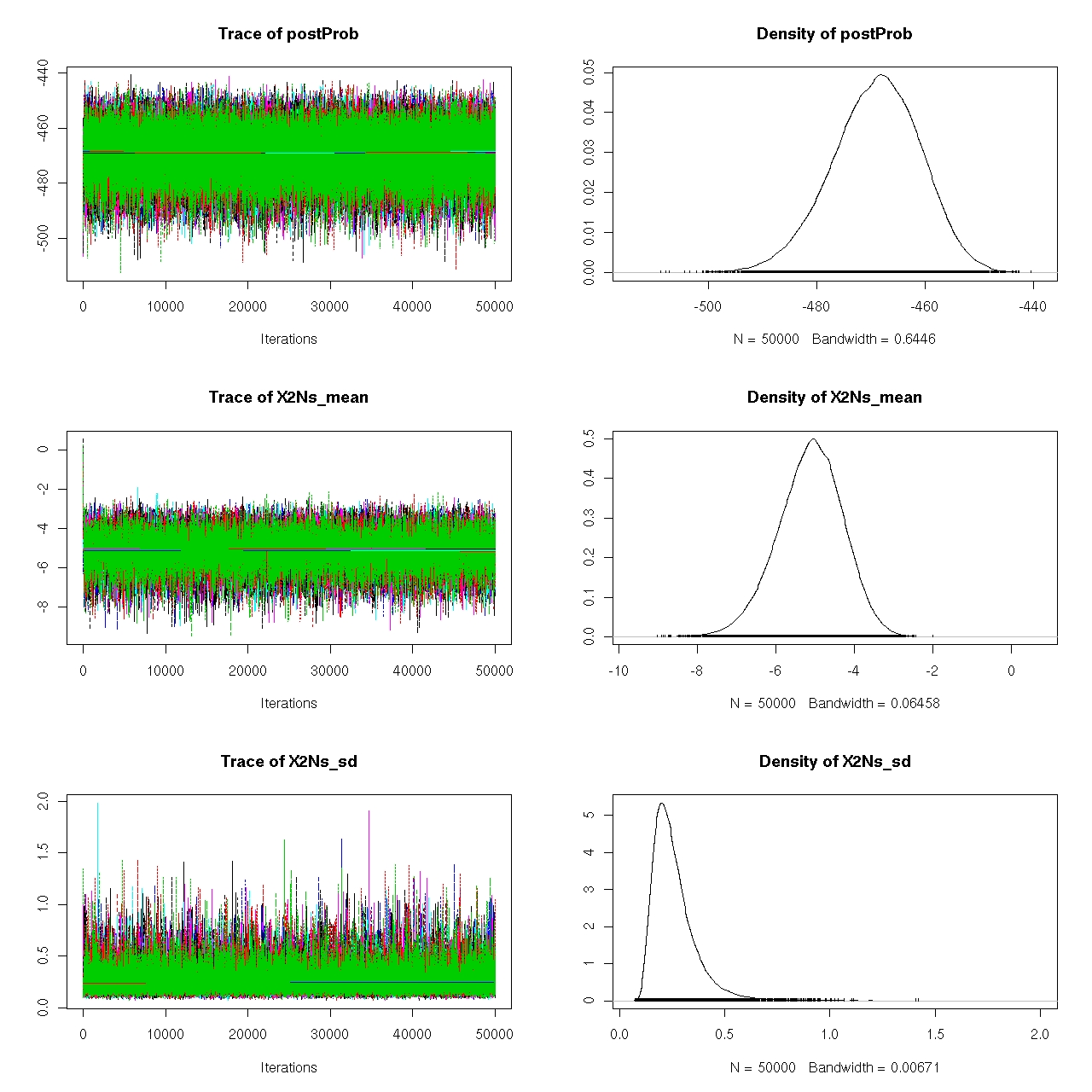
Typically a large number of iterations of the algorithm are run to ensure that
the Markov Chain has reached stationarity. For each dataset analyzed, we ran 9 separate
chains from overdispersed initial parameter values for 50,000 iterations. An example of
such a run of 9 chains is seen in Figure 2.8.
Convergence of our MCMC was monitored using the multivariate analog to
Gelman's potential scale reduction factor ˆ
R [12], which uses the independence of mul-
tiple chains to assess convergence by combining terms corresponding to the variance
between chains with those corresponding to the variance within chains. An example
of convergence using this metric is given in Figure 2.9, where one can see the scale
reduction factor quickly converging to 1.0. Once convergence was established, the first
10,000 iterations of each MCMC chain were considered burn-in and discarded, while the
remainder were retained for use in estimation.
Figure 2.8: MCMC output from one dataset. Nine independent chains are run from
overdispersed starting points and are shown here in individual colors. Displayed are the joint posterior
probability ("postProb"), µ ("X2Ns mean"), and σ ("X2Ns sd"), over the 50,000 iterations for the
case of UC regions using EA+AA pooled samples. Shown in the right hand panel are the marginal
distributions of each of the parameters. Convergence of our chains can be seen here by the relatively
consistent bands traced by the model parameters among chains.
Maximum Likelihood Estimates [AK]
The Hierarchical Bayesian MCMC model described in Section 2.12 treats the
mean selection coefficient µ as a random variable and allows calculation of its expected
last iteration in chain
last iteration in chain
last iteration in chain
Figure 2.9: Convergence plots for MCMC simulations. Shown here is the reduction in
the [12] scale reduction factor ("shrink factor") ˆ
R over the course of our MCMC iterations for the case
of UC regions using EA+AA pooled samples. Values close to 1.0 indicate convergence of the MCMC to
the posterior distribution of our parameters. Plot labels as in Figure 2.8.
value and variance. A less computationally intense and perhaps more conventional
approach can be used to derive the Maximum Likelihood (ML) point estimate of the
selection coefficient α where the likelihood of the data is, as before, the product of the
individual SNP probabilities given in Equation 2.3 but the SNPs are assumed to be
independent and identically distributed with a common selection coefficient α. That is,
we find the value of α that maximizes the likelihood
Following the methods of [13] we have numerically maximized Equation 2.7
to determine these ML estimates for our various genomic regions and population sub-
samples. The results comparing the ML estimates to the MAP estimates from the full
Bayesian model are shown in Table 2.5. It can be seen that the agreement between the
two methods is quite good so that our conclusion about the strength of selection on the
ultraconserved elements is not dependent on our Bayesian methods.
Table 2.5: Estimates of the selection coefficient using Bayesian and MaximumLikelihood methods MAP: Maximum A Posteriori estimate for mean value of selection coefficient
based on hierarchical Bayesian MCMC. ML: Maximum Likelihood point estimate for the selection
coefficient. Other symbols as in Table 2.3.
Effect of Linkage Disequilibrium
To investigate the possibility that linkage disequilibrium (LD) had an effect on
the derived allele frequency spectra, and hence my estimates of the selection coefficients
for the categories of sites examined, I performed calculations on subsets of the segre-
gating sites found in the pooled EA and AA samples analyzed above. For the Seattle
SNPs data, I chose 50 random subsets of the nonsynonymous and intron segregating
sites such that each subset had at most one segregating site per gene. For the UC and
UF sites I chose 50 random subsets such that each subset had at most one segregating
site per UX element. Thus the segregating sites in any of these subsets should have no
LD. For the UC sites I also chose 50 random subsets containing the same number (105)
of segregating sites as in the one-per-UX subsets of UC sites, but this time without
regard to the UX element of a site.
For each subset I calculated the ML estimate of the selection coefficient as
described in Section 2.14. The distribution across the subsets for each class is shown in
Figure 2.10. The median values of the subsets (listed in the caption of Figure 2.10) are
very close to the ML values for the EA+AA pooled samples (shown in Figure 2.10 and
listed in Table 2.5) with the largest effect being about a 15% reduction in the estimated
strong negative selection coefficient for the UC category. But this category has the
largest variance and the interquartile range of its subsets is completely consistent with
the its distribution in Figure 2.1. I am thus confident that my essential conclusion about
the selection coefficients in the different categories is not an artifact of LD.
ML Selection Coefficient
Figure 2.10: Selection Coefficient Estimates without Linkage Disequilibrium.
Boxplots of the distributions of Maximum Likelihood (ML) estimates of the selection coefficient, in units
of 2Nes, derived from 50 subsamples (for each category) of the segregating sites in the pooled EA+AA
samples are shown. The NonSyn and Intron subsamples include only one SNP per gene in the Seattle
SNPs data set. The UF and UC-noLD subsamples include at most one SNP per UX. The UC-rand
subsamples had the same number of SNPs as UC-noLD, but were chosen without replacement from UC
SNPs without regard to UX. The ML estimates for the full set of EA+AA samples in each category are
shown as thin red lines. The median values (-5.2, -4.4, -1.5, -1.3, -0.16) for the subsets are consistent
with the distribution of values in Figure 2.3, indicating that the latter are not strongly dependent on
linkage disequilibrium in the respective regions of segregating sites.
Ascertainment Effects [AK]
Ultraconserved elements of the human genome were identified through the
criterion of 100% sequence homology among species.
Since polymorphisms within
species are apt to be confused with fixed differences between species when single se-
quence comparisons are used, one would expect ultraconserved elements to contain
fewer polymorphisms than non-ascertained genomic regions even under the neutral
model. Furthermore, one would expect those polymorphisms that are present in ul-
traconserved elements of the genome to be segregating at lower frequencies than those
in non-ultraconserved regions, since intermediate and higher frequency polymorphisms
are more likely to be mistaken for fixed differences between species. Since our estimation
of selection coefficient uses information from the frequency spectrum of segregating poly-
morphism, these biases might mimic the effects of selection on ultraconserved regions
of the genome.
To quantify the strength of this ascertainment bias in our data, we performed
extensive coalescent simulation of the ultraconserved element identification process, to
examine the extent to which selection of ultraconserved elements alone can skew the
site frequency spectrum under neutral models. We used Hudson's "ms" program [32] to
perform the simulations under the standard neutral model (SNM). Our procedure con-
sisted of simulating 100,000 unlinked genomic regions from 96 individuals (representing
our human samples) and 1 outgroup lineage (representing a chimp sequence), with a
species divergence time of 5 units of 4Ne generations (about 5 million years assuming
Ne = 10,000 and a 25 year generation time), and a fixed value of θ (4Neu = 0.5).
We then split these 100,000 unlinked regions into those that were "ultraconserved" vs.
"non-ultraconserved" by comparing our outgroup sequence to one randomly selected
individual from our ingroup and finding those regions that had zero fixed differences in
the two-sequence comparison.
Distributions of Tajima's D [75] for our two classes of region are shown in the
left panel of Figure 2.11. The bias imposed by selection of the ultraconserved genomic
regions on Tajima's D results in a shift in the frequency spectrum towards rare alleles for
ultraconserved elements but the bias is quite small. Under the standard neutral model
we do not see values of Tajima's D that are as extreme as we observed in our data
(Table 2.3). Other demographic models incorporating population expansions yielded
similar results (data not shown).
Additionally we estimated the strength of selection α using ML estimates as
in Section 2.14, for the separately pooled sets of simulated "ultraconserved" and "non-
ultraconserved" polymorphisms. These simulations were repeated 10,000 times for the
standard neutral model (SNM) yielding the distributions shown in the right panel of
(Figure 2.11).
A fairly large difference between simulated ultraconserved and non-
ultraconserved sequences is observed. Ascertainment of ultras results in a negative shift
in estimates of the strength of selection, even under neutrality. In order to correct for
this ascertainment bias, we applied the procedure described in Section 2.17.
ML Selection Coefficient
Figure 2.11: Effect of Ascertainment Bias of Ultraconserved Elements onTajima's D and Estimates of Selection Coefficient.
Coalescent simulations were
performed using the standard neutral model (SNM) as described in the text, which were then split into
"ultraconserved" (ultras) and "non-ultraconserved" (non-ultra) subsets based on the absence/presence
of fixed differences in a two-sequence comparison between the outgroup sequence and a randomly chosen
ingroup sequence. Left panel shows boxplots of Tajima's D statistic, indicating that scertainment of the
ultraconserved elements has only a weak effect of biasing Tajima's D downward. Right panel shows box-
plots of Maximum Likelihood estimates of the selection coefficient, in units of 2Nes. If uncorrected, the
ascertainment bias for ultras results in an apparent negative selection coefficient for neutrally evolving
Correcting for Ascertainment Bias [AK]
As noted in Section 2.16, identification of the ultraconserved elements on the
basis of no divergence between species will impact the expected site frequency spec-
trum at those loci, even under the neutral model. To obtain accurate estimates of the
strength of selection at UC regions we modified our likelihood function (Equation 2.3
and Equation 2.4) to directly correct for this ascertainment bias. Following the general
framework of Nielsen et al. [51], we assume that our ascertainment was performed in
a subsample, size d, of our final sample, size n, where the derived allele frequency at
segregating site k was ik, such that the probability of ascertainment (probability of
choosing d ancestral alleles) is
In our case d = 1, corresponding to sampling the ancestral allele at our single genomic
reference sequence. With this probability in hand, using Bayes rule we can write down
the ascertainment corrected version of Equation 2.3 (suppressing the dependence on
sample size, but emphasizing that the bias is dependent on the site k). The probabil-
ity of observing a SNP segregating with derived allele frequency ik, conditional upon
ascertainment and the strength of selection α is
P r(ik α)P r(Asck ik, α)
P r(ik Asck, α) =
where the denominator is simply the normalization factor
P r(j α)P r(Asck j, α).
Our corrected likelihood function can then be expressed as
P (Data Asc, α) =
This ascertainment corrected likelihood function was tested using the coales-
cent simulation scheme described in Section 2.16. As can be seen in Figure 2.4, this
procedure returns the expected value of our estimates of the strength of selection back to
zero. Subsequently, all estimations done for UC regions, both Bayesian and Maximum
Likelihood, use this ascertainment corrected formulation.
A comparison of the ML estimates for the ultraconserved regions with and
without correction in various samples is given in Table 2.6. The correction reduces the
estimate for the UC regions by about 10-20%.
Table 2.6: Ultraconserved Element Ascertainment Bias Correction in Esti-mates of the selection coefficient. Maximum Likelihood point estimates for the selection
coefficient in the ultraconserved regions with (UC-corr) and without (UC-uncor) correction for the as-
certainment bias. The correction reduces the estimate by about 10-20%. Other symbols as in Table 2.3.
Evolution of Human Accelerated
Regions is GC-Biased
As noted in the Introduction, I enriched the genomic DNA from 11 individu-
als among the Yoruba from Ibidan, Nigeria (YRI samples) for 40kb neighborhoods of
the top 49 Human Accelerated Regions [59] (HARs) (hereinafter "harseq1-49"), and 13
similar control regions not containing HAR elements (hereinafter "ctlreg50-62") using
a microarray hybridization technique. Using ABI SOLiD [6] high throughput sequenc-
ing technology I obtained sufficient coverage in the target regions of the resulting short
(35bp and 50bp) sequencing reads to restrict my analysis to genotype calls at positions
where I had at least 35-fold coverage for an individual, to ensure accurate genotyping.
I determined the frequency of the derived (non-ancestral) allele in my set of 22 chro-
mosomal samples for all the resulting segregating sites (i.e. sites where not all samples
have the same allele).
I analyzed these segregating site frequencies in several ways. First, I compared
the frequency spectra of two subsets of my segregating sites: those comprising W2S
mutations (where the ancestral allele is either A or T, and the derived allele is either
G or C) versus the S2W mutations. Next, I compared the ratios of these different
classes of mutations to the same ratios for fixed substitutions that have arisen on either
the human or chimp lineages since our common ancestor ∼5 million years ago. For
both of these analyses I tested the strength of my results across the full scale of my
regions, and also performed the tests on the data pooled across my 49 genomic regions.
Finally, I examined the pattern of spatial variation of derived allele frequencies in search
of evidence for a selective sweep. Results for harseq regions and ctlreg regions were
compared to each other and to a set of 62 genic regions resequenced in the same 11 YRI
individuals by the Seattle SNPs project [4].
My key conclusions reinforce the notion that a bias in fixation of GC basepairs
is at play in the HAR neighborhoods. The use of the present tense ("is at play") in the
previous sentence is intentional, for I have two significant results. On the one hand, I
confirmed the historical GC-bias for fixation, finding in 10 of the 49 HAR neighborhoods
that fixed differences are more likely than polymorphic sites to show this bias. But in
my more novel result I also found that there is a similar GC-bias towards higher derived
allele frequencies at polymorphic sites alone. The high derived allele frequencies at these
GC-biased SNPs make them likely candidates for eventual fixation. I found this ongoing
bias in 11 cases, only 1 of which also shows historical GC-bias. Thus, almost half of HAR
regions (20) are currently undergoing, or have historically undergone, biased fixation of
GC alleles. This pattern strongly suggests that selectively neutral forces, such as biased
gene conversion, have helped to shape many of the genomic regions containing HARs
and could have influenced the fixation of a large number of GC alleles in the HAR
I also used my resequencing data to search for signals of a recent selective
sweep, which could have indicated that one or more of the HAR substitutions had been
subject to recent positive selection in the human population. In that analysis, I found
that only weak signals of that kind remain, possibly due to millions of years of decay.
It may be noteworthy that 3 of the 5 regions with those signals are also significant in
one of the two GC-bias tests.
The following sections provide more details of these results and describe the
methods used to derive them. In this work I collaborated with Andrew Kern who
implemented the coalescent simulations to determine p-values for the SweepFinder test
described below. Another collaborator in this work was Katherine Pollard who provided
the substitution rate matrix used in simulations to validate the p-values of the MK test
described below.
Results of HAR Neighborhood Analysis
Weak-to-Strong Mutations are Being Swept to Higher Derived
Allele Frequencies
When the HARs were first described, a strong W2S substitution bias was noted
in the human-specific substitutions in these elements [59, 60]. This bias was extremely
pronounced in HARs 1,2,3, and 5, but also noticeable as a general trend in the entire
set 1-49. This evidence suggested that biased gene conversion (BGC) could have had
an historical role in the evolution of the HARs. Here I analyze my list of segregating
sites in the 40kb HAR neighborhoods to determine if such bias is still ongoing in the
human population. In each region, I separately computed the derived allele frequency
spectra for the W2S mutations and the S2W mutations. I then tested for an offset in
the spectra between the two categories with a two-sided Mann Whitney U (MWU) test.
This test has been shown to have good power to detect fixation bias [3].
I found a significant (p ≤ 0.05) difference in 11 out of 49 harseq regions (Table
3.1). In all 11 significant harseq regions, the offset was for the W2S mutations to be
segregating at higher derived allele frequencies than S2W. This implies that regardless
of the rate of introduction of W2S or S2W mutations, it is the W2S mutations that are
more likely to reach high frequency and eventually fix in the human population. This
is certainly consistent with a mechanism of gene conversion that favors selection of G
or C alleles from a heterozygote or some other selective force generally favoring higher
GC content. The novel features of this result are that it indicates that this process is
ongoing and not confined to the core 100–400bp HAR elements.
This ongoing W2S fixation bias distinguishes the harseq regions from ctlreg
regions and Seattle SNPs regions. Significant MWU tests were observed at none of
ctrlreg50-62 (Table A.2) and five out of 62 Seattle SNPs regions (Table A.3), one of which
has higher derived allele frequencies in S2W compared to W2S mutations. Applying
the MWU test to simulations of a neutral coalescent model as described in Section 3.2.7
showed that the p-values from this test accurately reflect the fraction expected by chance
from a neutrally evolving locus.
The two harseq regions with the greatest offset were harseq21 and harseq34
(Figure 3.1). Note that across these two 40kb regions, the ratio of W2S to S2W segregat-
ing sites is not extreme; it is the W2S shift towards higher frequency in the population
that is significant. These ratios are consistent with the smoothed ratios reported in
the top several thousand conserved candidate HAR elements [59] even though my 40kb
regions do not comprise largely conserved regions.
It is natural to theorize that BGC will be a stronger driving force in areas
of high recombination and studies have shown there to be a good correlation with the
male recombination rate in particular [17]. I examined the recombination rates in the
enclosing 1Mb windows as determined by the deCODE project [41]. Harseq21 is an
outlier in that it is contained in a genomic region of extremely high recombination rate
(male 4.29 cM/Mb, sex-averaged 3.43 cm/Mb, in contrast to genome-wide averages of
0.93 cM/Mb and 1.29 cm/Mb respectively). But this is not true of harseq34 (0 male and
1.42 cm/Mb sex-averaged). For the remainder of the regions with a significant p-value
harseq21 segregating sites spectra. AT to GC vs. GC to AT mutations
fraction of sites
derived allele frequency (count of 22)
harseq34 segregating sites spectra. AT to GC vs. GC to AT mutations
fraction of sites
derived allele frequency (count of 22)
Figure 3.1: Frequency offset of weak-to-strong vs. strong-to-weak mutations.
MWU test is strongly significant for harseq21 (upper panel) and harseq34 (lower panel). This reflects
the fact that the derived allele frequency spectrum for weak-to-strong mutations (dark bars) is offset
towards higher frequencies compared to strong-to-weak mutations (light bars). N: count of segregating
sites of the indicated category in the region.
on the MWU test, the rates vary. An additional (not unrelated) factor that has been
strongly correlated with biased substitutions is chromosomal position near telomeres
[17]. With the exception of harseq1 this is not the case for the regions with significantly
shifted W2S spectra (Table 3.1).
I also performed the MWU test for the shift in W2S sites toward higher fre-
quencies after pooling all the segregating sites in my 49 harseq regions, and found a
p-value < 10−10. By contrast, the test was not significant (p = 0.26) for the pooled
data in my 13 control regions, thereby controlling for possible systematic bias in my
sequencing and genotyping techniques. I thus conclude that in many of the neighbor-
hoods of the top 49 HARs there is an ongoing force driving W2S mutations to higher
frequency in the human population.
Weak-to-Strong Mutations are More Likely to Have Become
Fixed Differences
Since the HARs were essentially defined based on fixed differences between
the human and chimp reference genomes in otherwise strongly conserved elements [59],
I compared such human/chimp fixed differences to the segregating sites in my human
samples. My set of fixed differences was based on high quality base calls from the
reciprocal best alignments [38] of human and chimp genomes. I further restricted this
list to the locations within my regions for which I had the above-mentioned 35-fold
coverage for an individual in my sample. Finally, I removed from this initial fixed
difference list those positions that I found to be segregating in my samples, or that
appeared in the dbSNP129 database [71] (see Section 3.2.6). The latter two filters
removed 6.7% of the fixed differences at high coverage positions. Since I do not have
information on sites that are segregating in the chimp population, I could not remove
those, but would expect the number to be similarly small.
I separated the mutations in my segregating site set into the categories: W2S,
S2W, and neither. I similarly divided the set of fixed differences, regardless of whether
the substitution occurred on the chimp or human lineage. As in reference [17], I per-
formed a variant of the McDonald-Kreitman (MK) test to compare the W2S:S2W ratios
in the sets of mutations and the sets of substitutions as described in Section 3.2.6.
I found a significant (p ≤ 0.05) difference between the substitution patterns
of segregating versus fixed sites in 11 of the 49 harseq regions (Table 3.2). In all but
one (harseq39) of these 11, the fixed substitutions had relatively more W2S mutations
(compared to S2W) from the ancestral form than did the segregating sites. Four of the
11 fell in the 40kb neighborhoods of the top 11 HARs, and indeed the strongest result
(p = 0.00015) was for harseq1. This is not surprising, since the HAR1 element has 18
fixed differences, all W2S [60]. By contrast, none of the ctlreg regions and nine out of
62 Seattle SNPs regions had a significant p-value on this test (Tables A.2 and A.3).
All of the nine significant Seattle SNPs regions had a higher W2S:S2W ratio in fixed
differences than in segregating sites. Thus, the harseq regions have a much stronger
signal for historical fixation bias than my control regions and a somewhat stronger
signal than the genic Seattle SNPs regions. Applying the MK test to simulations of a
neutrally evolving primate phylogeny (see Section 3.2.7) showed that the p-values from
this test accurately reflect the fraction expected by chance from a neutrally evolving
I also recapitulate and expand the finding [59] that this bias towards W2S fixa-
tion is associated with telomeres, since 7 of the 11 significant regions under the MK test
were found either in the karyotype band containing a telomere or the one immediately
adjacent. (This count includes the two cases of harseq19 and harseq36 from chromosome
2 that fall adjacent to the ancestral telomeric fusion event at 2q14.1.) Although many
of the 11 regions (including ones near telomeres) have elevated recombination rates, it
is also worth noting that 5 of the 11 are in regions with much lower than average male
recombination rates (including the two near the chromosome 2 fusion site, and harseq11
One noteworthy negative result from the MK test, (and the MWU test as
well) is harseq2. It had been noted [59] that the core HAR2 element showed a strong
bias towards W2S fixations, and that this extended to a region of ∼1kb. Here I find
no significant signal for either the MK or MWU test in my 40kb neighborhood of
that element (Table A.2). Another noteworthy negative result on these tests is the
harseq6 region, which has an extremely elevated rate of mutation as estimated either
by nucleotide diversity [76] or by the number of segregating sites [80] (Table A.1), but
apparently no strong bias towards weak-to-strong fixation (Table A.2).
Although the MK test, like the MWU test, is consistent with the mechanism
of BGC favoring fixation of G or C alleles, in fact only one of my regions (harseq1) had
significant results in both tests. Since the original identification of these elements as
HARs depended on substitutions fixed on the human lineage, it is not surprising under
the assumption of BGC to find that a bias towards W2S fixation is associated with
the HAR neighborhoods. The complementary evidence from the MWU test (a total of
20 of my 49 test regions are W2S-significant on one test or the other) indicates that
the ongoing bias in favor of W2S mutations has also probably led to human specific
substitutions in otherwise conserved elements.
The Scale of Fixation Bias towards Weak-to-Strong Mutations
Because BGC is posited to operate on a scale much smaller than the 40kb of my
target sequencing regions, perhaps operating at localized recombination hotspots, and
because the (100–400bp) HAR elements at the core of my target regions were suspected
of arising in part due to BGC [59], I wanted to test whether the MWU and MK signals
depended on these core elements. I therefore performed the same tests after masking
out the central 500bp, 1kb, 5kb or 10kb of each region.
I found that signals of both ongoing and historical fixation bias are fairly robust
to removing sequences including and flanking the core HAR element. For the MWU
test, all but two (harseq1, harseq18) of the 11 regions that were significant at the 5%
level for the MWU test were still significant at that level with the central 5kb omitted.
Seven of the 11 remained significant even with 10kb omitted (Table 3.1). For the MK
test, the results were slightly more sensitive to masking. Considering the 11 regions with
a significant result on that test (including the one favoring S2W fixation), 9(7) of these
were still significant with the central 1kb(5kb) masked out (Table 3.2). I conclude that
the evolutionary forces behind these results is not confined to the small HAR elements
themselves, but rather that any bias in the substitutions found in the HARs is likely a
byproduct of the forces acting at a larger scale.
To test whether there might be other localized elements within the 40kb regions
driving these results I performed the tests under a set of fifteen overlapping 5kb masks
(centered at a 2.5kb spacing along each region). Among the 11 MWU significant regions,
5 were still significant at 10% under this regime, while 3 completely lost significance (p
> 20%) for at least one such mask (Table 3.1). Of the 11 MK significant regions, 5
were still significant at 10% (including harseq1) under this regime, while 1 completely
lost significance (p > 20%) under at least one mask (Table 3.2). It is worth noting that
the harseq1 result reflects the fact that of the 105 segregating sites I found in that 40kb
neighborhood, 71 were S2W and only 19 W2S (Table A.2).
I conclude from this set of tests that the evolutionary forces behind W2S
fixation bias are not necessarily highly local. If fixation bias relies on recombination
hotspots and BGC, I have to posit that such hotspots extend over a long range of bases,
or are somehow temporally and spatially variable.
No Significant Evidence for Selective Sweeps
For each of the studied regions, I used the SFS to calculate two population
genetic statistics that can sometimes indicate positive selection: Tajima's D [75], which
is based on the folded SFS, and Fay and Wu's H [23]. Neither of these statistics exceeded
the value of ±2 in any region (Table A.1). I next compared the distributions of these
two statistics in the 49 harseq regions and the 13 ctlreg regions, to those for the same
population (YRI) in 104 genic regions resequenced by Seattle SNPs (see Section 3.2.7). I
found the ctlreg regions to be indistinguishable from the Seattle SNPs for these statistics,
while the harseq regions were only mildly more negative for Tajima's D (Wilcoxon rank
sum p-value = 0.08) and not significantly different for H (Figure 3.2). These results
strongly suggest that the site frequency spectrum in harseq regions is indistinguishable
from that found in either my control regions (ctlreg), or in the Seattle SNPs data set.
Thus there is no reason to believe that harseqs represent some kind of genomic outlier
with respect to recent selective events.
To test for evidence of a selective sweep, I analyzed the spatial variation of de-
rived allele frequencies at the segregating sites from my 22 chromosomal samples in each
of the target 40kb regions using the SweepFinder program. This software determines a
composite likelihood ratio (CLR) statistic comparing the hypothesis of a complete selec-
tive sweep at the location to the null hypothesis of no sweep using Test 2 from Nielsen
et al. [52]. I tested along a grid of 1000 points in each target region. This test has been
shown to be robust to demographic deviations from the standard neutral model in its
ability to use an arbitrary background site frequency spectrum [82]. I tested with two
such backgrounds: the first from the pooled set of all the data in the 49 harseq regions
plus 13 ctlreg regions, the second from the same population (YRI) as my samples but
with frequencies taken from the Seattle SNPs resequencing data [4] for a large set (104)
of genic regions. It should be noted that using the SFS from my data as the background
harseq1to49 vs p2seasnpgenes Wilcoxon 2−sided p−value = 0.08156
ctlreg50to62 vs p2seasnpgenes Wilcoxon 2−sided p−value = 0.9931
harseq1to49 vs p2seasnpgenes Wilcoxon 2−sided p−value = 0.1303
ctlreg50to62 vs p2seasnpgenes Wilcoxon 2−sided p−value = 0.6303
Figure 3.2: Comparison of Population Genetic Statistics in harseq regions andSeattle SNPs genes. Boxplots show the distribution of Tajima's D, Fay and Wu's H in my test
regions (harseq1-49), my control regions (ctlreg50-62) and YRI samples sequenced in 104 Seattle SNPs
to define the neutral model should be particularly conservative in that I am testing any
given region for deviations from that neutral model. To determine the significance of the
maximum CLR values, we performed coalescent simulations of each target region and
ran the SweepFinder program on each simulated set of segregating sites as described in
Section 3.2.5. I report as a p-value the fraction of simulations of each target that had
a CLR greater than or equal to the actual maximum CLR for that target (Table A.2)
The harseq regions with the most significant five SweepFinder p-values are
listed in Table 3.3. These are nearly all at the 95% confidence level for either of the two
background distributions used, but I note that none are individually significant after a
conservative Bonferroni correction, given the 49 harseq regions that were tested. Since
these may nevertheless harbor mutations that were selected for in the human lineage,
here I briefly note some of their characteristics that can be seen in tracks from the UC
Santa Cruz Genome Browser (Figure 3.3).
Table 3.3: SweepFinder Hits Target regions with most significant p-values for SweepFinder.
Har,Sea refer to null model background frequency spectrum derived from all target regions or Seat-
tleSNPs respectively. RecA and RecM are the sex-averaged or male only recombination rates at the
target region. karyo is the chromosomal karyotype band where the target region is found.
Unlike the other four SweepFinder hits, which all contain introns or exons of
coding genes, harseq25 is in a gene "desert". The nearest known gene, approximately
1Mb away on chromosome 4, is ODZ3, which is a transmembrane signaling protein most
23 q24 q25 4q26 27
A harseq25
SweepFinder CLR on harseq resequencing. bgrnd sfs = seasnp. gridsize = 1000
Segregating sites from harseq resequencing. Reddish for higher derived frequencies
Placental Mammal Basewise Conservation by PhyloP
Human Accelerated Regions
B harseq9
SweepFinder CLR on harseq resequencing. bgrnd sfs = seasnp. gridsize = 1000
Segregating sites from harseq resequencing. Reddish for higher derived frequencies
UCSC Genes Based on RefSeq, UniProt, GenBank, CCDS and Comparative Genomics
Placental Mammal Basewise Conservation by PhyloP
Human Accelerated Regions
C harseq11
SweepFinder CLR on harseq resequencing. bgrnd sfs = seasnp. gridsize = 1000
Segregating sites from harseq resequencing. Reddish for higher derived frequencies
UCSC Genes Based on RefSeq, UniProt, GenBank, CCDS and Comparative Genomics
Placental Mammal Basewise Conservation by PhyloP
Human Accelerated Regions
D harseq16
SweepFinder CLR on harseq resequencing. bgrnd sfs = seasnp. gridsize = 1000
Segregating sites from harseq resequencing. Reddish for higher derived frequencies
UCSC Genes Based on RefSeq, UniProt, GenBank, CCDS and Comparative Genomics
Placental Mammal Basewise Conservation by PhyloP
Human Accelerated Regions
E harseq24
SweepFinder CLR on harseq resequencing. bgrnd sfs = seasnp. gridsize = 1000
Segregating sites from harseq resequencing. Reddish for higher derived frequencies
UCSC Genes Based on RefSeq, UniProt, GenBank, CCDS and Comparative Genomics
Placental Mammal Basewise Conservation by PhyloP
Human Accelerated Regions
Figure 3.3: SweepFinder Composite Likelihood Ratio (CLR) in genomic con-text. For the indicated harseq regions, the SweepFinder results are shown along with the segregating
sites from my sequencing – more reddish for those with higher derived allele frequencies. Other tracks
show introns and exons of known genes and evolutionary conservation. The CLR peaks are not strongly
associated with the core HAR elements.
highly expressed in brain. Note that harseq25 also has a significant result on the MWU
test discussed above.
Evidence for a sweep in the harseq9 region is intriguing because it encompasses
the 42-codon long, second exon of the PTPRT gene, a phosphatase with possible roles
in the central nervous system. However, the human amino acid sequence of this exon
matches the other primates chimp, gorilla, and orangutan, except where chimp has an
obviously non-ancestral Thr>Ala substitution. The human sequence does have a single
G>A substitution near the 3' splice site just upstream of this exon, but it falls in a
position between the polypyrimidine (Py) tract and the AG acceptor site, for which the
consensus sequence across many splice sites is evenly divided among the 4 nucleotides.
The location of harseq11 on chromosome X places its evidence for a sweep in
the first intron of the 2.4Mb long dystrophin gene DMD. The evidence for a sweep in
harseq16 is offset to one end of its region, about 20kb from an apparent pseudogene
comprising a single coding exon with a 270-codon open reading frame (ORF) that is
probably derived from the Poly-A binding protein PABPC1.
The harseq24 region encompasses the second through fourth exons of the
SKAP2 gene with the strongest evidence for a sweep about 10kb from the closest exon,
but closer to a LINE transposable element that is present also in chimp, orangutan, and
rhesus macaque (but lost in gorilla).
Although I found only weak evidence for selective sweeps, and none that seems
to point directly to a mutation in a core HAR element based on the position of the
SweepFinder peak CLR values, it is important to note that while having the advantage
of robustness to demography and recombination rate, my tests would not likely have
power to detect sweeps that occurred beyond the last ∼200,000 years [82].
Methods for HAR Neighborhood Analysis
Sample Data Genomic DNA Selection
Genomic DNA for my samples was obtained from the NHGRI Sample Repos-
itory for Human Genetic Research distributed by the Coriell Institute for Medical Re-
search [Camden NJ] [1]. All of the 11 samples were chosen from the Yoruba from Ibidan
Nigeria (YRI) HapMap population. In particular, the samples were chosen as a subset
of the Seattle SNPs P2 panel [4]. The Seattle SNPs PGA-VDR (and Coriell repository
numbers were): DY01(NA18502), DY03(NA19223), DY04(NA19201), DY17(NA19143),
DY18(NA18517), DY19(NA18856), DY20(NA19239), DY21(NA18871), DY22(NA19209),
DY23(NA19152), DY24(NA19210). Sample preparation as described below was similar
for all samples, except that prior to processing, the DY01,DY03,DY04 samples were
subject to whole genome amplification (WGA) using the Repli-G Kit (Qiagen N.V, The
Netherlands) according to manufacturer's specifications. It was found that WGA caused
a loss of coverage in some isolated target regions, most notably in the 28kb section of
the harseq1 region with coordinates hg18:chr20:61,183,966–61,212,244, except for the
core HAR1 element at chr20:61,203,919-61,204,081.
Target Regions and Nimblegen Enrichment Array Design
The primary target regions consisted of 20kb extensions in both directions
from the 49 most statistically significant Human Accelerated Regions (HARs) identi-
fied as having a 5% false discovery rate [60]. Additional 40kb control regions were
chosen in neighborhoods of 13 of the set of 34,498 vertebrate conserved elements that
had extremely low likelihood ratio test (LRT) scores used to define the HARs. The
enrichment arrays were obtained from Nimblegen Systems (Madison WI) who designed
the probes on their 385K array based on my specifications of the coordinates of the 62
target genomic regions (Table A.1). Probes were chosen to tile the target regions from
both DNA strands. The design process avoided probes in highly repetitive sequences as
described previously [53, 5]. The fraction of bases in the target regions covered by the
probes ranged from 98% (harseq12) to 65% (harseq4) with a median of 88%. Details of
probed bases are available upon request.
At the time that I designed the enrichment array the main alternative tech-
nology for genomic DNA enrichment was to use oligonucleotide probes in solution. A
solution based method presumably would have better kinetic properties than the array
based method. However, the main drawback is cost. Synthesizing individual oligonu-
cleotides at a cost even as low as $0.10 per base would be prohibitively expensive to
cover target regions encompassing 2M bases. A commercially available alternative from
Agilent Technologies was also available based on their array technology in which they
separated the probes from the array after fabrication. This approach was successfully
used for enrichment of sets of exons in the human genome [61] but the cost was still
relatively high, since this technology provided 55,000 probes for about $10,000. Com-
pared to the 385,000 probes on the Nimblegen array (at about $1,000 per array) this
would have been much more expensive to cover my target regions, even considering the
fact that one order of Agilent probes would have sufficed to enrich DNA from all of my
SOLiD Barcoded Library Preparation
The library preparation of the samples for SOLiD (Applied Biosystems, Fos-
ter City, CA) sequencing generally followed the manufacturer's protocols for barcoded
SOLiD System 2.0 Fragment Library Preparation (samples DY01,DY03,DY04) and
SOLiD System 3.0 Barcoded Fragment Library Preparation (remaining samples), with
changes as necessary for enrichment on the Nimblegen arrays as noted in the following:
Samples were sheared to approximately 100bp using the Covaris S2 System Program B
(Covaris Inc, Woburn, MA). End repair was performed with End-It DNA End-Repair
Kit (Epicentre Biotechnologies, Madison, WI) per manufacturer's instructions. Single
stranded oligos for the P1 and P2-barcoded SOLiD adaptors were ordered from In-
vitrogen Corporation and annealed per the SOLiD protocol to form double stranded
adaptors, which were ligated to the end-repaired DNA fragments using the Quick Lig-
ation Kit (New England BioLabs, Ipswich, MA) per manufacturer's directions, leaving
a nick at the 3' end of each genomic DNA strand where the 5' end of the adaptor
was not phosphorylated. Samples DY01,DY03,DY04 were size selected to 150∼250bp
from a 6% polyacrylamide gel and purified via ethanol precipitation. This was followed
by nick translation and ligation mediated PCR (LMPCR) amplification (6 cycles) in a
combined reaction per the SOLiD protocols using Takara ExTaq polymerase (Takara
Bio, Madison, WI). After dividing into 10 aliquots, an additional 10 cycles of ExTaq
LMPCR amplification were performed on these samples in preparation for array hy-
bridization. Samples DY17-DY20 were first nick translated without amplification using
Pfu polymerase (Stratagene, La Jolla, CA). Samples DY21-DY24 were nick translated
and ExTaq LMPCR amplified (6 cycles). Quantitation using a DNA 2100 BioAnalyzer
(Agilent Technologies, Waldbronn, Germany) showed that the PCR associated with nick
translation prior to size selection mainly served to amplify the nick translated adaptors.
After the nick translation and any initial LMPCR, all of samples DY17-DY24 were size
selected on an E-Gel SizeSelect 2% agarose gel (Invitrogen) per manufacturer's instruc-
tions. These size selected samples were then ExTaq LMPCR amplified (6, 9 or 10 cycles)
in preparation for array hybridization.
Array hybridization to the Nimblegen arrays was performed on the Nimble-
gen Hybridization System 4 station under Mix Mode "B" for 64 to 70 hours using the
Nimblegen Sequence Capture Kit per manufacturer's instructions. Prior to hybridiza-
tion, samples DY21-24 were pooled to a total of 5.7µg. All the other samples were
hybridized individually, in amounts ranging from 1.9µg to 8.0µg per sample. For com-
petitive hybridization to probes on the array that might nonselectively bind repetitive
DNA, Human Cot-1 DNA (Invitrogen) that had been Covaris sheared to approximately
100bp was added to the hybridization mix in a 5:1 ratio by weight. Additionally, to
block the adaptor ends of the denatured, single stranded DNA fragments from binding
to each other, a 10:1 molar excess of adaptor oligos (P2 with an unused barcode sequence
and P1) was also added. At the completion of hybridization, the slide was washed with
the Nimblegen Sequence Capture Wash and Elution kit per manufacturer's directions,
and the enriched DNA was eluted with 350µL of 75◦C purified water using an affixed
SA200 SecureSeal Hybridization Chamber (Grace Bio-Labs, Bend OR). A secondary
elution with an additional 350µL was also taken. Quantitative real-time PCR (qPCR)
was performed on the eluted material to determine the rough fraction of target DNA
and to compare the primary and secondary elutions. For this purpose qPCR amplicons
within the target were compared to amplicons not in the target regions. It was gener-
ally found that the primary elution captured more than 95% of the target DNA (data
not shown). By normalizing to pre-enrichment material, and taking into account the
fact that the 2.1Mbp target region comprised approximately 0.1% of the entire human
genome, it was estimated that more than 35% of the eluted material fell in the target
regions (data not shown).
The eluted material was ExTaq LMPCR amplified (samples DY01 for 19 cy-
cles, samples DY03-04 for 15 cycles, pooled samples DY21-24 for 10 cycles, samples
DY17-20 for 12 cycles,) in preparation for the emulsion PCR step of SOLiD sequenc-
ing that was performed in the UC Santa Cruz Genome Sequencing Center. Samples
DY01,DY03,DY04 were processed with the SOLiD Version 2 system, producing 35 bases
of sequence information for each read. The remaining samples were processed with the
SOLiD Version 3 system, producing 50 bases of sequencing information for each read.
Sequence Mapping, Filtering, and Genotyping
The 35mer (DY01,DY03,DY04) or 50mer (remaining samples) sequencing reads
were mapped to the whole human genome using the bwa program [43] which generates
mappings and associated quality scores in the sam format [44] that can be processed
with the samtools suite. The bwa program is aware of the colorspace nature of the
SOLiD sequencing reads, and uses a dynamic programming algorithm to infer the best
nucleotide sequence for the read [43]. All reads were also mapped to the DNA of the
Epstein-Barr Virus, which was used to transform the Coriell cell lines from which the
supplied genomic DNA was extracted. For the female samples, the Y chromosome was
excluded from the mapping. For the male samples, the pseudo-autosomal region of the
Y chromosome was excluded from the mapping. The set of mappings for each sample
was then filtered to the regions covered by the probes on the Nimblegen enrichment
array described above. To eliminate spurious pileups caused by overamplification of
particular molecules in the library preparation process, the mapped reads were further
filtered to select at most 4 reads from each strand at a given genomic starting posi-
tion. Where there were more than 4, the 4 with the highest total read quality (not
the best mapping quality, which would bias against reads containing non-reference al-
leles) from the SOLiD instrument were selected. Between 40% and 60% of the reads
for a given sample were successfully mapped, and of those reads, between 33% and
48% mapped to bases covered by the probes on the enrichment array (Table 3.4). For
samples DY01,DY03,DY04 about 50% of the latter reads were lost in the "maximum 4
per strand" pileup elimination step, while only 11% to 23% were lost in this step in the
remaining samples (Table 3.4 and Figure 3.4). This was likely due to the difference in
LMPCR cycles used for the different samples as noted above.
To determine the coverage at each position in the target region and the con-
sensus genotypes for each sample, the command "samtools pileup -v" was used with
default parameters for its consensus calling model. Possible confounding of the geno-
types due to contamination by paralogous sequences was avoided in two ways. First,
as noted, only genotypes at positions delimited by the Nimblegen probes were used in
the analysis and these probes were designed to avoid repetitive sequences. Second, the
bwa mapping algorithm assigns low mapping quality to reads that are not genome-wide
unique, and the samtools consensus caller requires high mapping quality. To filter SNPs
from among the not homozygous reference genotypes, "samtools.pl varFilter" was run
with default parameters, except that the maximum read depth was set to 425, because
with up to 4 reads of length 50 on each strand, it was possible to get coverage of 400.
This command filters out potential SNPs when more than 2 fall within a 10bp window,
on the grounds that there might be an insertion/deletion event rather than separate
SNPs, and also filters out reads with RMS mapping quality value less than 25. A sim-
ilar quality filter was applied to the genotype calls that were homozygous reference.
Because of stochastic variation in the composition of reads from the two chromosomes
of each diploid individual, low coverage might cause an erroneous homozygous call in
a true heterozygote. Therefore a further filter restricted the subsequent analysis to the
SNP or homozygous reference calls made for a sample only at positions for which the
coverage was 35 or greater. For each target region, the count of the union of such posi-
tions across all samples is listed in Table A.1. As shown in Figure 3.5, the vast majority
of the segregating sites that remain after the application of my 35X coverage filter are
in Hardy-Weinberg Equilibrium, with only 0.3% having a p-value less than 0.05.
Table 3.4: HAR Region Mapping Statistics M: million reads. Total: the total number of
reads obtained for a given sample. Mapped: the subset of Total that mapped successfully to the human
genome. mapFrac is Mapped/Total. Probed: the subset of Mapped that mapped to the regions defined
by the probes on the Nimblegen enrichment array. probeFrac is Probed/Mapped. 4Best: the subset of
Probed that remain after filtering to allow at most 4 reads from each strand at each starting position in
the genome. 4bestFrac is 4Best/Probed. Sample DY02 was not included in the analysis because 97%
of its on-target reads were removed in the "4best" pileup elimination step.
Derived Allele Frequencies and SweepFinder
For purposes of all subsequent analysis, an ancestral allele at each position
in the target regions was determined from the Enredo-Pecan-Ortheus (EPO) pipeline
[54, 55] as published on the 1000 Genomes website [2]. This pipeline determines the
common ancestor of human and chimp at a locus by considering alignments of the
human, chimp, orangutan, and rhesus macaque genomes.
Figure 3.4: HAR Region Mapping Statistics by Sample. Graphical representation
of the data in Table 3.4. Although the starting number of reads ("Total") varied widely across the
samples, roughly the same number of reads ("4Best") were used for genotyping each sample. As noted
in Table 3.4 sample DY02 was excluded from the analysis.
Histogram of HWE p−values (two.sided)
N−total= 5835 N−pval<0.01= 1 N−pval<0.05= 17 N−pval<0.10= 56
umber of segsitesn
Figure 3.5: Histogram of Hardy-Weinberg Equilibrium Test. Histogram of the p-
values obtained in a 2-sided test for Hardy-Weinberg equilibrium across all of the SNPs used in the
analysis of my test (harseq) and control (ctlreg) regions. The vast majority conform to the HWE
From the sets of filtered genotype calls in the 11 diploid samples as described
above all the segregating sites were selected. A set of filters was applied to this list to
produce the final set of segregating site derived (i.e. non-ancestral) allele frequencies
(DAFs) for all downstream analyses. To avoid skewing the DAFs towards higher fre-
quencies, segregating sites with less than 8 chromosomal samples were eliminated. Also
eliminated were any positions with more than 2 alleles among the reference, ancestral,
or sample alleles, or where the ancestral allele was not determined by the EPO pipeline.
Lowercase values of the EPO ancestral allele, which result from various cases without
complete evidence in all species were not eliminated.
The SweepFinder program [52] was applied to the allele frequencies for the
final list of segregating sites to determine the composite likelihood ratio (CLR) of a
selective sweep at each one of a grid of 1000 positions across each target region. The
model used in this program requires a background derived allele frequency spectrum.
Two such backgrounds were used. First, all of the DAFs from all filtered segregating
sites in my sample were aggregated and used as input to the command "SweepFinder -
f", which accounts for missing data using a Broyden-Fletcher-Goldfarb-Shanno (BFGS)
algorithm. I refer to this as the "harseq" background. A second, presumably more
neutral background was obtained from the African-Derived (AD) YRI subset of 24
individuals in the Seattle SNPs P2 panel. The DAFs for all segregating sites in all 104
genes resequenced for this panel by Seattle SNPs [4] were included. As for the harseq
background, the "seasnp" background was obtained with the command "SweepFinder
-f" applied to these DAFs. The resulting "seasnp" frequency spectrum ran from 1 to 47
and was reduced to a spectrum running from 1 to 21, as needed by SweepFinder with my
data, by hypergeometric weighting the relevant components of the input Xj(j = 1.47)
allele frequencies at each target Yi(i = 1.21) allele frequency.
Dividing by the sum of the Yi in Eqn 3.1 produces a valid frequency spectrum
that sums to 1. A similar hypergeometric weighting was also required to reduce the
spectrum to a range from 1 to 19 for the harseq1,2 and ctlreg60 regions. In the latter
regions missing data reduced the maximum number of samples at the segregating sites
to 20. The reasoning behind the hypergeometric weighting can be understood from
an example. Consider a site for which, among 48 samples, there are 6 derived and
42 ancestral alleles.
At this site a subsample of 22 from the 48 samples has some
probability P3,6 of having 3 derived and 19 ancestral alleles that can be calculated as
follows. Think of the site as an urn with 6 "D" balls and 42 "A" balls. There are 48�
possible subsamples. For each of these subsamples there are 6� ways to choose 3 "D"
balls and 42� ways to choose 19 "A" balls from the urn. So the probability P
hypergeometric factor 6� 42�/ 48�. Now if there are M
6 such sites, the expected number
of such sites for which the subsample has 3 derived alleles is given by N3,6 = M6P3,6.
For other sites with at least 3 (of 48) derived alleles and at least 19 (of 48) ancestral
alleles similar calculations can be made and then summed to get the total expected
number of sites with 3 (of 22) derived alleles N3 = P MjP3,j. Dividing both sides by
the total number of sites yields equations in the form of Equation 3.1. The additional
normalization step is required because it is possible for many of the subsampled sites
to yield either 0 or 22 derived alleles, but we are only interested in sites which are
segregating in the subsample.
MWU and MK tests on Harseq and Ctlreg Regions
To determine if mutations from an ancestral weak (A or T) basepair to a
strong (G or C) basepair (W2S mutations) are more likely to spread in the popula-
tion represented by my samples, I compared W2S segregating sites to S2W segregating
sites for each target region and for the aggregate set of segregating sites. I performed
a Mann-Whitney U (MWU) test for a difference between the W2S and S2W derived
allele frequency spectra. The test was performed in the R language with the command
"wilcox.test (paired=FALSE, alternative=two.sided)". The resulting "location" param-
eter was normalized to 22 samples and is positive if W2S mutations are segregating at
higher frequencies than S2W. The resulting p-values are in Table A.2.
To determine if relatively more W2S mutations fixed along the human or chimp
lineages than are segregating in the human population represented by my samples, I
first determined the high mapping quality chimp reference bases that differ from the
human reference using reciprocal best alignments of the chimp and human genomes
[38]. This set was then restricted to the positions in my target regions for which I had
a genotype call for at least one sample with read depth of coverage of 35 or greater as
discussed above. From this set of fixed differences I removed any for which the EPO
ancestral allele was not determined as discussed above, or for which I had a segregating
site, or which appeared in dbSNP release 129 [71]. The remaining fixed differences as
well as the segregating sites were divided into W2S or S2W (or other). A McDonald
Kreitman-like (MK) test on the resulting 2x2 contingency table was performed in the
R language with the command "fisher.test (alternative=two.sided)". The resulting p-
values are in Table A.2. For the significant cases it was easy to determine from the data
in the contingency table if the fixed differences favored S2W mutations relatively more
than the segregating sites (column "S2W" in Table 3.2).
For the target regions with significant p-values on either the MWU or MK
tests, I tested whether the significance was due to a restricted locus within the region,
by removing all segregating sites and fixed differences under a mask of a given size at a
given position within the region and rerunning the test with the remaining data (Table
3.1 and Table 3.2).
MWU and MK Tests on Seattle SNPs Regions and Simulations
I downloaded the data for the 104 genes resequenced with the Seattle SNPs P2
panel. The genotypes for my 11 YRI samples (which are a subset of the P2 panel) and
the coordinates for the genotyped segregating sites were obtained from the global "pret-
tybase" file mapped to UCSC hg18 coordinates. The total set of positions genotyped
was obtained from the individual gene "genbank" files by excluding the features defined
as "Region not scanned for variation" and aligning the remaining regions to the hg18
coordinates of the full extent of the genic region sequenced specified in the associated
"ucscDataFile". Given these coordinates and the genotypes at the segregating sites,
the same techniques as described above for my resequencing data was applied to derive
ancestral alleles and human/chimp fixed differences, and to perform the MWU and MK
My data was derived from (probed) regions of a relatively tight size distribu-
tion (Table A.1). By contrast, the sizes of Seattle SNPs variation-mapped genic regions
varied widely. Some were rather small and contained few segregating sites. Therefore, I
included only genic regions with a minimum of 10kb variation-mapped and a minimum
of 40 segregating sites. Additionally, a small number of the genic regions were excluded
because of data missing from the "prettybase" file or because there were no associated
high quality reciprocal best human-chimp differences as described above, possibly be-
cause of paralogous genes in one or the other lineage. The remaining set of results for
the MWU and MK tests on 62 genic regions (Table A.3) were used for comparison to
my 49 harseq regions.
To determine if the p-values for the MWU and MK tests were accurate, I
also conducted the tests on sets of simulated data. For the MWU test, I performed
coalescent simulations using Hudson's ms program [32]. For each simulation I generated
22 samples at 85 segregating sites (the average number of W2S plus S2W segregating
sites in the 49 harseq target regions) and then randomly assigned the sites as either
W2S or S2W in Bernoulli trials using the W2S:S2W ratio from the 49 harseq regions
of 2057:2114. After calculating the MWU test p-value for each simulation, the fraction
of simulations with p-value less than a given value was computed, as well as the subset
of that fraction in which the W2S spectrum was offset towards higher derived allele
frequencies (Figure 3.6).
Fraction of Simulations by MWU−test p−value
all (slope = 0.998)
W2S (slope = 0.513)
Figure 3.6: Accuracy of MWU Test p-values. For a given p-value the fraction of neutral
model simulations having that p-value or better on the MWU test is shown. Red circles: all simulations
with a better p-value. Blue squares: the simulations with a better p-value for which the weak-to-strong
(W2S) spectrum is offset towards higher frequency. Regression lines are shown with the slope indicated
in the legend. For a given p-value the W2S-biased simulations comprise about half of all simulations.
For the MK test, for each simulation I separately derived a set of human-
chimp fixed differences and a set of segregating sites. The fixed differences were derived
using the phyloBoot program from the PHAST package [72]. I used a phylogenetic
model and substitution rate matrix derived from 4-fold degenerate amino-acid coding
synonymous sites across the genome as an unbiased neutral model. The equilibrium
GC-content of this model was adjusted to reflect the genome-wide average GC-content.
From the primate sequences so generated, I extracted positions containing a human-
chimp difference that could also be unambiguously assigned an ancestral allele based on
the macaque allele at that position. Each simulation used 335 such sites, (the average
number of fixed differences in the 49 harseq target regions) which were divided based on
whether they were W2S or S2W (or other). The segregating sites for each simulation
were derived from 101 (the average total number of segregating sites in the 49 harseq
target regions) Bernoulli trials, randomly dividing them as W2S or S2W (or other)
according the corresponding ratios in the fixed differences from all of the phyloBoot
simulations. After calculating the MK test p-value for each simulation, the fraction of
simulations with p-value less than a given value was computed, as well as the subset
of that fraction for which the ratio of W2S:S2W was higher for the simulated fixed
differences than for the simulated segregating sites (Figure 3.7).
Fraction of Simulations by MK−test p−value
all (slope = 0.865)
W2S (slope = 0.426)
Figure 3.7: Accuracy of MK Test p-values. For a given p-value the fraction of neutral
model simulations having that p-value or better on the MK test is shown. Red circles: all simulations
with a better p-value. Blue squares: the simulations with a better p-value for which the weak-to-strong
(W2S) fraction is relatively higher in fixed differences than segregating sites. Regression lines are shown
with the slope indicated in the legend. The p-values are conservative in that they overestimate the
fraction of simulations at a given significance level. For a given p-value the W2S-biased simulations
comprise about half of all simulations.
In the era of comparative genomics, strong signals of conservation across mul-
tiple species serve as signposts that can indicate regions where evolutionary forces may
be preserving functional elements that are subject to purifying selection. By contrast,
signals of positive selection pointing to adaptive changes in one lineage are harder to
find, often employing sets of polymorphic sequences from multiple individuals of the
same species.
In this work I have addressed both of these aspects of the evolutionary history
of the human genome. In my work on the Ultraconserved Elements (UCEs) I employed
resequencing data for a large number of samples that was obtained using classical meth-
ods based on PCR followed by capillary electrophoresis Sanger sequencing. From this
resequencing data I identified polymorphic positions and then derived and analyzed the
derived allele frequency (DAF) spectrum of these polymorphisms. The results of my
analysis clearly show that these elements, taken as a whole, are under strong selective
constraint. This constraint is in fact much stronger than that at play in protein coding
sequences. This result effectively laid to rest any speculation that these elements are
merely mutational cold spots, lacking any likely function. An important challenge that
was overcome in this work was the inherent ascertainment bias in the definition of these
elements wherein polymorphic positions at high derived allele frequency are likely to
prevent a region from being defined as ultraconserved. An especially striking aspect of
my results was that the bases immediately flanking the UCEs are apparently subject to
much weaker selective forces.
Although these conclusions about the UCEs are important, they are only ap-
plicable to the UCEs as an aggregate because the analysis of the DAF spectrum was
only possible using all the polymorphisms found across these elements. Most individual
UCEs have zero, one or two SNPs. Thus it was not possible to make statements about
the strength of selection of particular elements, nor to infer if any are in fact more likely
to be functional than others.
By contrast, my analyses of the HARs were applied separately to a 40kb neigh-
borhood of each region. I exploited the two recently developed techniques of genomic
enrichment and high throughput sequencing to characterize the polymorphism in a sin-
gle human population across these neighborhoods of the 49 HARs (harseq regions). I
investigated the harseq regions because the HARs were defined based on a presump-
tion that the human lineage specific fixed differences therein might have arisen due to
adaptive evolutionary forces. On the other hand, it has been emphasized by some that
the presumably evolutionarily neutral mechanism of biased gene conversion (BGC) can
influence the frequency spectra at polymorphic positions, or cause fixation of alleles in
a way that partially mimics the action of adaptive evolution. Indeed, fixation bias was
noted in connection with the limited set of human specific alleles for some of the HARs
when they were first described [59].
With the extensive novel polymorphism in my samples, I was able to carefully
characterize fixation bias — both historical and ongoing — in the harseq regions and
to conduct tests for recent selective sweeps across these regions. Like my resequencing
data for the UCEs, my harseq resequencing data eliminates issues of SNP ascertainment
bias that could have skewed previous investigations of polymorphism near HARs.
Consistent with published reports [59, 17, 26], I found evidence of historical
W2S fixation bias in harseq regions. Using a MK test, I compared the proportion of
W2S mutations among already fixed substitutions on the human or chimp lineage to
that among the still segregating sites in my samples. I found that 11 of the 49 regions
show statistically significant evidence of historical bias in allele fixation, with all but
one favoring W2S fixation. These results strengthen and expand previous findings by
identifying signals for W2S bias in much larger regions flanking the core HAR regions
in an ascertainment-free population sample.
But my work goes beyond previous approaches by also looking at ongoing
W2S fixation bias in the segregating site frequency spectrum. I performed a MWU
test using only sites that are still segregating in the human population, separating out
W2S from S2W mutations. This second test is designed to detect a phenomenon of bias
that is currently driving W2S mutations to higher frequency in the population than
S2W mutations. I found statistically significant evidence for this bias (and none in the
opposite direction) in the regions flanking 11 of 49 HARs.
For both tests, I showed that the core HAR element is generally not the main
source of the signal that was detected, since the signal usually remains strong even
when I mask out the central 1kb or even 5kb of the region. This is not consistent
with BGC due to a recombination hot spot that has remained in the same location for
millions of years, because the length scale of the effect of BGC is set by the length of
the heteroduplex tract formed during recombination that needs to be repaired, which
is thought to be ∼500bp (e.g. [11, 65, 25]). However, it is consistent with a model in
which the location of recombination hotspots drift fairly rapidly over evolutionary time
scales, but may be denser in some regions [64, 58, 48, 15, 57].
It is noteworthy that there was little overlap in the regions identified by these
two tests, one for older W2S fixations and the other for present day forces toward
fixation, with a total of 20 found in one or the other.
This is consistent with the
hypothesis that the regional focus of BGC, which may be recombination hot spots,
drifts significantly on a time scale of many hundreds of thousands or millions of years.
Another explanation for W2S fixation bias near HARs is selection for increased
GC-content or individual fitness-improving GC alleles. To investigate these hypotheses
and to attempt to disentangle the possible roles of BGC and positive selection in shaping
the HARs, I applied a recently developed powerful method for detecting selective sweeps.
Selection was previously investigated in much larger (∼500kb) regions using more sparse
polymorphic loci [82]. That study found 101 regions with strong evidence for a selective
sweep within 100kb of a known gene. Here, I found only weak evidence for selection
comprising 5 possible candidates for such sweeps among 49 target regions. As we are
dealing with a lineage-specific evolutionary period of about 5 million years, and these
tests can only see back a few hundred thousand years, it is quite possible that the original
signal for selective sweeps in these regions has already decayed beyond our ability to
recognize it in human population genetic data.
Consistent with the idea that HAR regions may have experienced positive se-
lection too long ago to be detected with population genetic methods, very few positively
selected regions in the human lineage have been identified to date, despite the existence
of numerous public databases. Selective sweeps that have been identified have typically
been the product of very recent events in human history, such as dairy farming affect-
ing the lactase gene [8] or climate differences influencing a salt sensitivity variant [78].
Such environmental or cultural changes result in differences in the genetic makeup of
disparate human populations, and such differences can be exploited to find evidence of
recent, possibly still ongoing, selective sweeps.
Despite the evidence that the unusually high level of recent substitution in the
more extreme HAR elements such as HAR1 is at least partly due to the non-selective
process of BGC, there is ample evidence that some of these genomic elements remain
functional, and thus that the effect of BGC was to mutationally stress but not destroy
these elements. HAR1 shows a very strong pattern of compensatory substitutions within
its RNA helix structures, indicating a selective force to maintain these helix structures.
The W2S substitutions all strengthen the RNA helices of HAR1, and in one case, a
substitution appears to extend one of them. Thus, although the nominally non-selective
GC-biased evolutionary force that I have documented may reduce the fitness advantage
of some HARs, it is also possible that it has enabled some of these regions to attain a
configuration subject to positive selection for higher fitness in humans.
In summary, I have investigated two sets of highly conserved genomic regions.
For both sets I have used polymorphism data from the present day human population
to elucidate evolutionary forces at work. I have shown that purifying selection is likely
preventing the UCEs from diverging in our species from the ancestral state, and that
some of the base substitutions now evident in the HARs are likely to be the result of a
process that favors fixation of mutations from weak to strong basepairs. As larger data
sets of human genetic variation become available it should be possible to expand these
results to the genome-wide scale.
Supplementary Tables
HAR Region Statistics. Characteristics of the target (harseq1-
49) and control (ctlreg50-62) regions in the HAR study. hg18pos: chromosome
coordinates in the hg18 human assembly. bpExp: the number of basepairs
used in the experimental analysis. This number starts with the count of bases
in the region that were included in probes in the Nimblegen array, but only
includes bases for which sequencing coverage of at least 35X was reached for
at least one sample, after removing pileups of more than 4 reads at the same
starting point. AncGC: the GC percentage of the ancestral bases in bpExp.
θπ: estimate of the neutral mutation parameter (= 4Neu x104) via nucleotide
diversity. θW : estimate of the neutral mutation parameter via the number of
segregating sites. tajD: measure of skew in the folded site frequency spectrum.
faywuH: measure of skew in the unfolded site frequency spectrum.
HAR Region Test Results
segsites (N): total number of
segregating sites from my samples. fixed diffs (N): number of positions for
which I had sufficient coverage to make a genotype call in at least one sample
that have a fixed difference between the human and chimp reference, exclud-
ing segregating sites and sites in dbSNP129.
w2s,s2w: subsets with weak-
to-strong or strong-to-weak mutations from the ancestral basepair. MWUp-
value,MWUoffset: p-value and estimated location offset (the latter normalized
to 22 samples and estimated under the assumption that w2s and s2w have
identical distributions) from Mann-Whitney U test comparing the frequency
spectra of segsites w2s vs s2w, with positive values indicating W2S mutations
shifted to higher derived allele frequencies. MKpval: p-value from McDonald-
Kreitman-like test comparing the counts in w2s,s2w categories of segregating
and fixed sites. SF: p-values for maximum CLR from SweepFinder run on the
region with a background SFS derived from segregating sites pooled from all
regions (Hpvalue) or from the same population segregating in Seattle SNPs
resequenced regions (Spvalue).
Seattle SNPs Gene Region MWU and MK Test Results
basepairs(Gene): total length of genic region. basepairs(Map): sum of base-
pairs in regions that were mapped for variation within genic region. AncGC:
the GC percentage of the ancestral bases in Map basepairs. segsites (N): to-
tal number of segregating sites in Map basepairs for my samples. fixed diffs
(N): number of positions in Map basepairs that have a fixed difference between
the human and chimp reference, excluding segregating sites and sites in db-
SNP129. w2s,s2w: subsets with weak-to-strong or strong-to-weak mutations
from the ancestral basepair. Other annotations as in Table A.2.
[1] Coriell cell repositories. http://ccr.coriell.org
[2] 1000 genomes: A deep catalog of human genetic variation. http://1000genomes.
org , August 2009.
[3] H. Akashi. Inferring the fitness effects of DNA mutations from polymorphism and
divergence data: statistical power to detect directional selection under stationarityand free recombination. Genetics, 151:221–238, Jan 1999.
[4] J.M. Akey, M.A. Eberle, M.J. Rieder, C.S. Carlson, M.D. Shriver, D.A. Nickerson,
and L. Kruglyak. Population history and natural selection shape patterns of geneticvariation in 132 genes. PLoS Biol., 2:e286, Oct 2004.
[5] T.J. Albert, M.N. Molla, D.M. Muzny, L. Nazareth, D. Wheeler, X. Song, T.A.
Richmond, C.M. Middle, M.J. Rodesch, C.J. Packard, G.M. Weinstock, and R.A.
Gibbs. Direct selection of human genomic loci by microarray hybridization. Nat.
Methods, 4:903–905, Nov 2007.
[6] Applied Biosystems. SOLiD System Brochure. System Brochure, Jun 2008.
[7] G. Bejerano, M. Pheasant, I. Makunin, S. Stephen, W.J. Kent, J.S. Mattick, and
D. Haussler. Ultraconserved elements in the human genome. Science, 304:1321–1325, May 2004.
[8] T. Bersaglieri, P. C. Sabeti, N. Patterson, T. Vanderploeg, S. F. Schaffner, J. A.
Drake, M. Rhodes, D. E. Reich, and J. N. Hirschhorn. Genetic signatures of strongrecent positive selection at the lactase gene. Am. J. Hum. Genet., 74:1111–1120,Jun 2004.
[9] C. P. Bird, B. E. Stranger, M. Liu, D. J. Thomas, C. E. Ingle, C. Beazley, W. Miller,
M. E. Hurles, and E. T. Dermitzakis. Fast-evolving noncoding sequences in thehuman genome. Genome Biol., 8:R118, 2007.
[10] M. Blanchette, W.J. Kent, C. Riemer, .L Elnitski, A.F.A. Smit, K.M. Roskin,
R. Baertsch, K. Rosenbloom, H. Clawson, E.D. Green, D. Haussler, and W. Miller.
Aligning multiple genomic sequences with the threaded blockset aligner. GenomeResearch, 14:708–715, 2004.
[11] H. L. Blanton, S. J. Radford, S. McMahan, H. M. Kearney, J. G. Ibrahim, and
J. Sekelsky. REC, Drosophila MCM8, drives formation of meiotic crossovers. PLoSGenet., 1:e40, Sep 2005.
[12] S.P. Brooks and A. Gelman. General methods for monitoring convergence of iter-
ative simulations. Journal of Computational and Graphical Statistics, 7:434–455,1997.
[13] C.D. Bustamante, J. Wakeley, S. Sawyer, and D.L. Hartl. Directional selection and
the site-frequency spectrum. Genetics, 159:1779–1788, Dec 2001.
[14] Francis S. Collins, Lisa D. Brooks, and Aravinda Chakravarti. A DNA polymor-
phism discovery resource for research on human genetic variation. Genome Re-search, 8:1229–1231, 1998.
[15] G. Coop, X. Wen, C. Ober, J. K. Pritchard, and M. Przeworski. High-resolution
mapping of crossovers reveals extensive variation in fine-scale recombination pat-terns among humans. Science, 319:1395–1398, Mar 2008.
[16] Jared A Drake, Christine Bird, James Nemesh1, Daryl J Thomas, Christopher
Newton-Cheh, Alexandre Reymond, Laurent Excoffier, Homa Attar, Stylianos EAntonarakis, Emmanouil T Dermitzakis, and Joel N Hirschhorn. Conserved non-coding sequences are selectively constrained and not mutation cold spots. NatureGenetics, 38:223–227, 2006.
[17] T.R. Dreszer, G.D. Wall, D. Haussler, and K.S. Pollard. Biased clustered substitu-
tions in the human genome: the footprints of male-driven biased gene conversion.
Genome Res., 17:1420–1430, Oct 2007.
[18] L. Duret and P.F. Arndt. The impact of recombination on nucleotide substitutions
in the human genome. PLoS Genet., 4:e1000071, May 2008.
[19] L. Duret and N. Galtier.
Comment on "Human-specific gain of function in a
developmental enhancer". Science, 323:714; author reply 714, Feb 2009.
[20] W. Enard, M. Przeworski, S. E. Fisher, C. S. Lai, V. Wiebe, T. Kitano, A. P.
Monaco, and S. Pbo. Molecular evolution of FOXP2, a gene involved in speechand language. Nature, 418:869–872, Aug 2002.
[21] B Ewing and P Green. Basecalling of automated sequencer traces using phred. II.
error probabilities. Genome Research, 8:186–194, 1998.
[22] B Ewing, L Hillier, M Wendl, and P Green. Basecalling of automated sequencer
traces using phred. I. accuracy assessment. Genome Research, 8:175–185, 1998.
[23] J. C. Fay and C. I. Wu. Hitchhiking under positive Darwinian selection. Genetics,
155:1405–1413, Jul 2000.
[24] R. A. Fisher. The Genetical Theory of Natural Selection. Clarendon Press, Oxford,
[25] L. Frisse, R. R. Hudson, A. Bartoszewicz, J. D. Wall, J. Donfack, and A. Di Rienzo.
Gene conversion and different population histories may explain the contrast be-tween polymorphism and linkage disequilibrium levels.
Am. J. Hum. Genet.,
69:831–843, Oct 2001.
[26] N. Galtier and L. Duret. Adaptation or biased gene conversion? Extending the
null hypothesis of molecular evolution. Trends Genet., 23:273–277, Jun 2007.
[27] N. Galtier, L. Duret, S. Glmin, and V. Ranwez. GC-biased gene conversion pro-
motes the fixation of deleterious amino acid changes in primates. Trends Genet.,25:1–5, Jan 2009.
[28] John H. Gillespie. Population Genetics: A Concise Guide. JHU Press, 2004.
[29] D Gordon, C Abajian, and Green P. Consed: a graphical tool for sequence finishing.
Genome Research, 8:195–202, 1998.
[30] E. Hodges, Z. Xuan, V. Balija, M. Kramer, M.N. Molla, S.W. Smith, C.M. Middle,
M.J. Rodesch, T.J. Albert, G.J. Hannon, and W.R. McCombie. Genome-wide insitu exon capture for selective resequencing. Nat. Genet., 39:1522–1527, Dec 2007.
[31] F. Hsu, W.J. Kent, H. Clawson, R.M. Kuhn, M. Diekhans, and D Haussler. The
UCSC known genes. Bioinformatics, 22:1036–46, 2006.
[32] Richard R. Hudson. Generating samples under a Wright-Fisher neutral model of
genetic variation. Bioinformatics, 18:337–338, 2002.
[33] Mark A. Jobling, Matthew Hurles, and Chris Tyler-Smith. Human Evolutionary
Genetics. Garland Publishing, 2004.
[34] N.L. Kaplan, R.R. Hudson, and C.H. Langley. The hitchhiking effect revisited.
Genetics, 123:887–899, Dec 1989.
[35] S. Katzman. Materials and Methods: Human genome ultraconserved elements are
ultraselected. Online Supporting Material, 2007. http://compbio.soe.ucsc.edu/papers/ultras meth v31.pdf
[36] S. Katzman, A.D. Kern, G. Bejerano, G. Fewell, L. Fulton, R.K. Wilson, S.R.
Salama, and D. Haussler. Human genome ultraconserved elements are ultraselected.
Science, 317:915, Aug 2007.
[37] Peter D. Keightley, Martin J. Lercher, and Adam Eyre-Walker.
widespread degradation of gene control regions in hominid genomes. PLoS Biology,3:e42, 2005.
[38] W. James Kent, Robert Baertsch, Angie Hinrichs, Webb Miller, and David Haus-
sler. Evolution's cauldron: duplication, deletion, and rearrangement in the mouseand human genomes. Proc Natl Acad Sci U S A, 100:11484–11489, 2003.
[39] A. D. Kern. Correcting the site frequency spectrum for divergence-based ascertain-
ment. PLoS ONE, 4:e5152, 2009.
[40] Y. Kim and W. Stephan. Detecting a local signature of genetic hitchhiking along
a recombining chromosome. Genetics, 160:765–777, Feb 2002.
[41] A. Kong, D. F. Gudbjartsson, J. Sainz, G. M. Jonsdottir, S. A. Gudjonsson,
B. Richardsson, S. Sigurdardottir, J. Barnard, B. Hallbeck, G. Masson, A. Shlien,S. T. Palsson, M. L. Frigge, T. E. Thorgeirsson, J. R. Gulcher, and K. Stefans-son. A high-resolution recombination map of the human genome. Nat. Genet.,31:241–247, Jul 2002.
[42] Gregory V Kryukov, Steffen Schmidt, and Shamil Sunyaev. Small fitness effect
of mutations in highly conserved non-coding regions. Human Molecular Genetics,14:2221–2229, 2005.
[43] H. Li and R. Durbin. Fast and accurate short read alignment with Burrows-Wheeler
transform. Bioinformatics, 25:1754–1760, Jul 2009.
[44] H. Li, B. Handsaker, A. Wysoker, T. Fennell, J. Ruan, N. Homer, G. Marth,
G. Abecasis, and R. Durbin. The Sequence Alignment/Map format and SAMtools.
Bioinformatics, 25:2078–2079, Aug 2009.
[45] G. Marais. Biased gene conversion: implications for genome and sex evolution.
Trends Genet., 19:330–338, Jun 2003.
[46] J. Maynard Smith and J. Haigh. The hitch-hiking effect of a favourable gene.
Genet. Res., 23:23–35, Feb 1974.
[47] J. Meunier and L. Duret. Recombination drives the evolution of GC-content in the
human genome. Mol. Biol. Evol., 21:984–990, Jun 2004.
[48] S. Myers, C. C. Spencer, A. Auton, L. Bottolo, C. Freeman, P. Donnelly, and
G. McVean. The distribution and causes of meiotic recombination in the humangenome. Biochem. Soc. Trans., 34:526–530, Aug 2006.
[49] Masatoshi Nei and Takashi Gojobori. Simple methods for estimating the numbers
of synonymous and nonsynonymous nucleotide substitutions. Molecular Biologyand Evolution, 3:418–426, 1986.
[50] D.A. Nickerson, V.O. Tobe, and S.L Taylor. Polyphred: automating the detection
and genotyping of single nucleotide substitutions using fluorescence-based rese-quencing. Nucleic Acids Research, 25:2745–2751, 1997.
[51] R. Nielsen, M. J. Hubisz, and A. G. Clark. Reconstituting the frequency spectrum
of ascertained single-nucleotide polymorphism data. Genetics, 168:2373–2382, Dec2004.
[52] R. Nielsen, S. Williamson, Y. Kim, M.J. Hubisz, A.G. Clark, and C. Bustamante.
Genomic scans for selective sweeps using SNP data. Genome Res., 15:1566–1575,Nov 2005.
[53] D.T. Okou, K.M. Steinberg, C. Middle, D.J. Cutler, T.J. Albert, and M.E. Zwick.
Microarray-based genomic selection for high-throughput resequencing. Nat. Meth-ods, 4:907–909, Nov 2007.
[54] B. Paten, J. Herrero, K. Beal, S. Fitzgerald, and E. Birney. Enredo and Pecan:
genome-wide mammalian consistency-based multiple alignment with paralogs.
Genome Res., 18:1814–1828, Nov 2008.
[55] B. Paten, J. Herrero, S. Fitzgerald, K. Beal, P. Flicek, I. Holmes, and E. Birney.
Genome-wide nucleotide-level mammalian ancestor reconstruction. Genome Res.,18:1829–1843, Nov 2008.
[56] L. A. Pennacchio, N. Ahituv, A. M. Moses, S. Prabhakar, M. A. Nobrega,
M. Shoukry, S. Minovitsky, I. Dubchak, A. Holt, K. D. Lewis, I. Plajzer-Frick,J. Akiyama, S. De Val, V. Afzal, B. L. Black, O. Couronne, M. B. Eisen, A. Visel,and E. M. Rubin. In vivo enhancer analysis of human conserved non-coding se-quences. Nature, 444:499–502, Nov 2006.
[57] A. D. Peters. A combination of cis and trans control can solve the hotspot conver-
sion paradox. Genetics, 178:1579–1593, Mar 2008.
[58] M. Pineda-Krch and R. J. Redfield. Persistence and loss of meiotic recombination
hotspots. Genetics, 169:2319–2333, Apr 2005.
[59] K.S. Pollard, S.R. Salama, B. King, A.D. Kern, T. Dreszer, S. Katzman, A. Siepel,
J.S. Pedersen, G. Bejerano, R. Baertsch, K.R. Rosenbloom, J. Kent, and D. Haus-sler. Forces shaping the fastest evolving regions in the human genome. PLoSGenet., 2:e168, Oct 2006.
[60] K.S. Pollard, S.R. Salama, N. Lambert, M.A. Lambot, S. Coppens, J.S. Peder-
sen, S. Katzman, B. King, C. Onodera, A. Siepel, A.D. Kern, C. Dehay, H. Igel,M. Ares, P. Vanderhaeghen, and D. Haussler. An RNA gene expressed duringcortical development evolved rapidly in humans. Nature, 443:167–172, Sep 2006.
[61] G.J. Porreca, K. Zhang, J.B. Li, B. Xie, D. Austin, S.L. Vassallo, E.M. LeProust,
B.J. Peck, C.J. Emig, F. Dahl, Y. Gao, G.M. Church, and J. Shendure. Multiplexamplification of large sets of human exons. Nat. Methods, 4:931–936, Nov 2007.
[62] S. Prabhakar, J. P. Noonan, S. Pbo, and E. M. Rubin. Accelerated evolution of
conserved noncoding sequences in humans. Science, 314:786, Nov 2006.
[63] S. Prabhakar, A. Visel, J.A. Akiyama, M. Shoukry, K.D. Lewis, A. Holt, I. Plajzer-
Frick, H. Morrison, D.R. Fitzpatrick, V. Afzal, L.A. Pennacchio, E.M. Rubin, andJ.P. Noonan. Human-specific gain of function in a developmental enhancer. Science,321:1346–1350, Sep 2008.
[64] S. E. Ptak, A. D. Roeder, M. Stephens, Y. Gilad, S. Pbo, and M. Przeworski.
Absence of the TAP2 human recombination hotspot in chimpanzees. PLoS Biol.,2:e155, Jun 2004.
[65] S. J. Radford, S. McMahan, H. L. Blanton, and J. Sekelsky. Heteroduplex DNA
in meiotic recombination in Drosophila mei-9 mutants. Genetics, 176:63–72, May2007.
[66] M. V. Rockman, M. W. Hahn, N. Soranzo, F. Zimprich, D. B. Goldstein, and G. A.
Wray. Ancient and recent positive selection transformed opioid cis-regulation inhumans. PLoS Biol., 3:e387, Dec 2005.
[67] Steve Rozen and Helen J. Skaletsky. Primer3 on the www for general users and
for biologist programmers. In S Krawetz and S Misener, editors, BioinformaticsMethods and Protocols: Methods in Molecular Biology., pages 365–386. HumanaPress, Totowa, NJ, 2000.
[68] P.C. Sabeti, D.E. Reich, J.M. Higgins, H.Z. Levine, D.J. Richter, S.F. Schaffner,
S.B. Gabriel, J.V. Platko, N.J. Patterson, G.J. McDonald, H.C. Ackerman, S.J.
Campbell, D. Altshuler, R. Cooper, D. Kwiatkowski, R. Ward, and E.S. Lander.
Detecting recent positive selection in the human genome from haplotype structure.
Nature, 419:832–837, Oct 2002.
[69] P.C. Sabeti, P. Varilly, B. Fry, J. Lohmueller, E. Hostetter, C. Cotsapas, X. Xie,
E.H. Byrne, S.A. McCarroll, R. Gaudet, S.F. Schaffner, and E.S. Lander. Genome-wide detection and characterization of positive selection in human populations.
Nature, 449:913–918, Oct 2007.
[70] S. A. Sawyer and D. L. Hartl. Population genetics of polymorphism and divergence.
Genetics, 132:1161–1176, 1992.
[71] S.T. Sherry, M.H. Ward, M. Kholodov, J. Baker, L. Phan, E.M. Smigielski, and
K. Sirotkin. dbSNP: the NCBI database of genetic variation. Nucleic Acids Res.,29:308–311, Jan 2001.
[72] A. Siepel and D. Haussler. Phylogenetic estimation of context-dependent substitu-
tion rates by maximum likelihood. Mol. Biol. Evol., 21:468–488, Mar 2004.
[73] Elizabeth M. Smigielski, Karl Sirotkin, Minghong Ward, and Stephen T. Sherry.
dbsnp: a database of single nucleotide polymorphisms. Nucleic Acids Research,28:352–355, 2000.
[74] J.N. Strathern, B.K. Shafer, and C.B. McGill. DNA synthesis errors associated
with double-strand-break repair. Genetics, 140:965–972, Jul 1995.
[75] F. Tajima. Statistical method for testing the neutral mutation hypothesis by DNA
polymorphism. Genetics, 123:585–595, Nov 1989.
[76] Fumio Tajima. Evolutionary relationship of DNA sequences in finite populations.
Genetics, 105:437–460, 1983.
[77] K. Tang, K.R. Thornton, and M. Stoneking. A New Approach for Using Genome
Scans to Detect Recent Positive Selection in the Human Genome. PLoS Biol.,5:e171, Jun 2007.
[78] E. E. Thompson, H. Kuttab-Boulos, D. Witonsky, L. Yang, B. A. Roe, and
A. Di Rienzo. CYP3A variation and the evolution of salt-sensitivity variants. Am.
J. Hum. Genet., 75:1059–1069, Dec 2004.
[79] B.F. Voight, S. Kudaravalli, X. Wen, and J.K. Pritchard. A map of recent positive
selection in the human genome. PLoS Biol., 4:e72, Mar 2006.
[80] G. A. Watterson. On the number of segregating sites in genetical models without
recombination. Theoretical Population Biology, 7:256–276, 1975.
[81] S. H. Williamson, R. Hernandez, A. Fledel-Alon, L. Zhu, R. Nielsen, and C. D. Bus-
tamante. Simultaneous inference of selection and population growth from patternsof variation in the human genome. Proc. Natl. Acad. Sci. U.S.A., 102:7882–7887,May 2005.
[82] S. H. Williamson, M. J. Hubisz, A. G. Clark, B. A. Payseur, C. D. Bustamante,
and R. Nielsen. Localizing recent adaptive evolution in the human genome. PLoSGenet., 3:e90, Jun 2007.
[83] A. Woolfe, M. Goodson, D. K. Goode, P. Snell, G. K. McEwen, T. Vavouri, S. F.
Smith, P. North, H. Callaway, K. Kelly, K. Walter, I. Abnizova, W. Gilks, Y. J.
Edwards, J. E. Cooke, and G. Elgar. Highly conserved non-coding sequences areassociated with vertebrate development. PLoS Biol., 3:e7, Jan 2005.
[84] S Wright. Evolution and the Genetics of Populations, volume Vol. 2: The Theory
of Gene Frequencies. University of Chicago Press, Chicago, 1969.
Source: https://compbio.soe.ucsc.edu/theses/Sol-Katzman-PhD-2010.pdf
B. Raj Kumar et al. / JGTPS/ 5(3)-(2014) 1827- 1832 Journal of Global Trends in Pharmaceutical Sciences Journal home page: www.jgtps.com A NEW VALIDATED STABILITY-INDICATING RP-HPLC METHOD FOR THE DETERMINATION OF TELBIVUDINE B. Raj Kumar1* Dr. K. V. Subrahmanyam2 Telbivudine 5'–triphosphate inhibits HBV DNA polymerase (reverse
Evidence-Based RegenerativeInjection Therapy (Prolotherapy)in Sports Medicine K. Dean Reeves, MD; Bradley D. Fullerton, MD, FAAPMR;and Gaston Topol, MD use of prolotherapy, which is also called regenerative injection ther-apy (RIT), is expected to greatly accelerate in the next decade. This . The treatment of sports injuries to the point of restoration of full chapter will cover the pathology of injury; the current treatment meth-